August 2011 – 0 FPS

As a warm up post, I’m going to talk about an important generalization of something that should be familiar to anyone’s who has made through a semester of calculus: Taylor series! (And if you haven’t seen these guys before, or are perhaps feeling a bit rusty, then by all means please head on over to Khan academy to quickly brush up. Go right ahead, I’ll still be here when you get back.)

Now this probably sounds like an awfully scary title for the first article in this miniseries about mathematics in graphics programming. Perhaps you’re right! But I’d like to think that graphics programmers are a tough bunch, and that using this kind of a name may indeed have quite the opposite effect of emboldening those cocky individuals who think they can press on and figure things out in spite of any frightening mathematical jargon.

Taylor Series

At the very heart of this discussion we are going to deal with two of the most important tasks any graphics programmer needs to worry about: approximation and book keeping. Taylor series are of course one of the oldest and best known methods for approximating functions. You can think of Taylor series in a couple of ways. One possibility is to imagine that they are successively approximating a given input function by adding additional polynomial terms to it. So the idea is that you can start with some arbitrary 1D function, let’s call it $f : R^1 \to R$ , and suppose that you are allowed the following two operations:

You can evaluate a function at 0.
You can take a derivative, $\partial_x f(x)$

Then, we can compute the Taylor series expansion of f about 0 in the usual way,

$f(x) = f(0) + (\partial_x f)(0) x + (\partial_{x} \partial_x f)(0) \frac{x^2}{2!} + (\partial_{x} \partial_x \partial_x f)(0) \frac{x^3}{3!} + ...$ and so on

If we’re really slick, we can save the first $k$ coefficients for these polynomials in a vector, call them say $a_0, a_1, a_2, ... a_{k-1}$ ., and then we can evaluate some approximation of f by summing up the first k terms in the above approximation:

$f(x) = a_0 + a_1 x + a_2 \frac{x^2}{2!} + a_3 \frac{x^3}{3!} + ... a_{k-1} \frac{x^{k-1}}{(k-1)!} + O(x^{k})$

Here is an animated gif showing the convergence of the Taylor series for the exponential function that I shamelessly ripped off from wikipedia:

Higher Dimensional Taylor Series

It is easy to adapt Taylor series to deal with vector valued functions in a single variable, you just treat each component separately. But what if the domain f was not one dimensional? This could easily happen for example, if you were trying to approximate something like a surface, a height field, or an image filter locally. Well, in this post I will show you a slick way to deal with Taylor series of all sizes, shapes and dimensions! But before I do that, let me show you what the ugly and naive approach to this problem looks like:

Suppose that $f (x,y) : R^2 \to R$ is a 2D scalar-valued function. Then, let us look for a best quadratic (aka degree 2) approximation to f within the region near $(0,0)$ . By analogy to the 1D case, we want to find some 2nd order polynomial $p(x,y)$ in two variables such that:

$p(x,y) = a_{00} + a_{10} x + a_{01} y + a_{20} x^2 + a_{11} xy + a_{02} y^2$

And:

$p(0,0) = f(0,0)$

$(\partial_x p)(0,0) = (\partial_x f)(0,0)$

$(\partial_y p)(0,0) = (\partial_y f)(0,0)$

$(\partial_{x} \partial_x p)(0,0) = (\partial_{xx} f)(0,0)$

$(\partial_{x} \partial_y p)(0,0) = (\partial_{xy} f)(0,0)$

$(\partial_{y} \partial_y p)(0,0) = (\partial_{yy} f)(0,0)$

Phew! That’s a lot more equations and coefficients than we got in the 1D case for a second order approximation. Let’s work through solving for the coefficient $a_{20}$: To do this, we take p and plug it into the appropriate equation:

$\left( \partial_{x} \partial_x (a_{00} + a_{10} x + a_{01} y + a_{20} x^2 + a_{11} xy + a_{02} y^2) \right) = 2 a_{20} = (\partial_{x} \partial_x f)(0,0)$

If we generalize this idea a bit, then we can see that for an arbitrary Taylor series approximation in 2D, the coefficient $a_{ij}$ is determined by the equation,

$a_{ij} = \frac{1}{i! j!} (\partial_{x^i y^j} f)(0,0)$

All this is well and good, but it has a few problems. First, the summation for p is quite disorganized. How are we supposed to keep track of which coefficients go where? If we want to store the coefficients of p on a computer, then we need some less ad-hoc method for naming them and packing them into memory. Second, it seems like this is going to be a headache to deal with 3 or more dimensions, since we’ll need to basically repeat the same sort of reasoning over and over again. As a result, if we want to start playing around with higher dimensional Taylor series, we’re going to need a more principled notation for dealing with higher order multivariate polynomials.

Tensors to the Rescue!

One such system is tensor notation! Though often maligned by mathematical purists. algebraic geometers, and those more modern algebraically savvy category theorists, tensors are a simple and effective notation that dramatically simplifies calculations. From a very simplistic point of view, a tensor is just a multidimensional array. The rank of the tensor is the number of different indices, each of which has a distinct dimension. In C-style syntax, you could declare a tensor in the following way:

  float vector[10];                          //A rank 1 tensor, with dimension (10)
  float matrix[5][5];                        //A rank 2 tensor, with dimensions (5, 5)
  float spreadsheet[ROWS][COLUMNS][PAGES];   //A rank 3 tensor, with dimensions (ROWS, COLUMNS, PAGES)
  float crazy_thing[10][16][3][8];           //A rank 4 tensor, with dimension (10, 16, 3, 8 )

We will usually write tensors as upper case letters. To reference an individual entry in this array, we will use an ordered subscript, like so:

$M_{ij}$

Which we can take to be equivalent to the C-code:

  M[i][j]

For the rest of the article, we are going to stick with this point of view that tensors are just big arrays of numbers. We aren’t going to bother worrying about things like covariance/contravariance (and if you don’t know what those words are, forget I said anything), nor are we going to mess around too much with operators like tensor products. There is nothing wrong with doing this, though it can be a bit narrow minded and it does somewhat limit the applications to which tensors may be applied. If it bothers you to think about tensors in this way, here is a more algebraic/operational picture of what a tensor does: much as how a row vector can represent a scalar-valued linear function, $R^n \to R$ (via the dot-product), a tensor can represents a multi-linear function, $R^n \times R^m \times ... \to R$ : that is, it takes in several vectors and spits out a scalar which varies linearly in each of its arguments.

That said, even if we just think about tensors as arrays, there’s still a number of useful, purely formal, operations that one can perform on tensors. For example, you can add them up just like vectors. If A and B are two tensors with the same dimensions, then we can define their sum componentwise as follows:

$(A + B)_{i} = A_{i} + B_{i}$

Where we take the symbol i to be a generic index here. The other important operation that we will need to use is called tensor contraction. You can think of tensor contraction as being something like a generalization of both the dot product for vectors, and matrix multiplication . Here is the idea: Suppose that you have two tensors $A, B$ with dimensions $(a_0, ... d, ... a_n), (b_0, ... d, ... b_m)$ and ranks n,m respectively and some index between them with a common dimension. Then we can form a new tensor with rank n + m – 1 by summing over that index in A and B simultaneously:

$C_{a_0, ..., a_n, b_0, ... b_n} = \sum_{i=0}^d A_{a_0, ..., i ..., a_n } B_{b_0, ... i, ... b_m}$

Writing all this out is pretty awkward, so mathematicians use a slick short hand called Einstein summation convention to save space. Here is the idea: Any time that you see a repeated index in a product of tensor coefficients that are written next to each other, you sum over that index. For example, you can use Einstein notation to write the dot product of two vectors, $x, y$ , as follows:

$x_i y_i = \sum \limits_{i=0}^d x_i y_i = x \cdot y$

Similarly, suppose that you have a matrix M, then you can write the linear transformation of a vector x by M in the same shorthand,

$y_j = M_{ji} x_i$

Which beats having to remember the rows-by-columns rule for multiplying vectors! Similarly, you can multiply two matrices using the same type of notation,

$(A B)_{i j} = A_{ik} B_{kj}$

It even works for computing things like the trace of a matrix:

$\mathrm{trace }(M) = M_{ii} = \sum \limits_{i} M_{ii}$

We can also use tensor notation to deal with things like computing a gradient. For example, we write the derivative of a function $f : R^n \to R$ with respect to the $i^{th}$ component as $\partial_i f$ . Combined with Einstein’s notation, we can also perform operations such as taking a gradient of a function along a certain direction. If $v$ is some direction vector, then the derivative of $f$ along $v$ evaluated at the point $x$ is,

$(\partial_i f)(x) v_i$

Symmetric Tensors and Homogeneous Polynomials

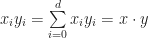
Going back to multidimensional Taylor series, how can we use all this notation to help us deal with polynomials? Well, let us define a vector $x = (x_0, x_1, ... )$ whose components are just the usual $(x, y, z ...)$ coordinate variables, and pick some rank 1 tensor A with appropriate dimension. If we just plug in x, then we get the following expression:

$A_i x_i = A_0 x_0 + A_1 x_1 + ...$

Which is of course just a linear function on x! What if we wanted to make a quadratic function? Again, using tensor contraction this is no big deal:

$A_{i j} x_{i} x_{j} = A_{0 0} x_0 x_0 + A_{0 1} x_0 x_1 + A_{1 0} x_1 x_0 + A_{1 1} x_1 x_1 + ...$

Neat! This gives us a quadratic multivariate polynomial on x. Moreover, it is also homogeneous, which means that it doesn’t have any degree 1 or lower terms sitting around. In fact, by generalizing from this pattern if we wanted to say store an arbitrary degree n polynomial, we could pack all of its coefficients into a rank n tensor, and evaluate by contracting:

$A_{i j k ... l} x_i x_j x_k ... x_l = A_{0 0 .... 0} x_0^n + A_{0 0 .... 1} x_0^{n-1} x_1 + ...$

But there is some redundancy here. Notice in the degree 2 case, we are assuming that the components of x commute, or in other words the terms $x_0 x_1, x_1 x_0$ are really the same and so we really don’t need to store both the coefficients $A_{10}$ and $A_{01}$ . We could make our lives a bit easier if we just assumed that they were equal. In fact, it would be really nice if whenever we took any index, like say $A_{i j k ... }$ and then permuted it to something arbitrary, for example $A_{j i k ...}$ , it always gave us back the same thing. To see why this is, let us try to work out what the coefficient for the monomial $x_{i_0} x_{i_1} .. x_{i_n}$ in the degree n polynomial given by $A_{i j k ... } x_i x_j x_k ...$ . Directly expanding using Einstein summation, we get a sum over all permutations of the indices $i_0, ... i_n$ :

$\sum \limits_{ \sigma \in \{ \mathrm{permutation of } i_0 ... i_n \} } A_{\sigma_0 \sigma_1 ... \sigma_n} x_{i_0} x_{i_1} ... x_{i_n}$

If we assume that all those $A_{...}$ coefficients are identical, then that above nasty summation has a pretty simple form: namely it is a multinomial coefficient! As a result, if we wanted to say find the coefficient of $x^2_0 x_1$ in $A_{i j k} x_i x_j x_k$, then we could just use the following simple formula:

$\frac{3!}{2! 1! 1!} A_{0 0 1} x^2_0 x_1 = { 3 \choose 2, 1, 0}$

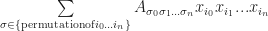
A tensor which has the property that its coefficients are invariant under permutation of its indices is called a symmetric tensor, and as we have just seen symmetric tensors provide a particularly efficient method for representing homogeneous polynomials. But wait! There’s more…

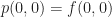
If we pick $A_{0 0 1} = (\partial_{001} f)(0)$ , then the above formula is almost exactly the right formula for the Taylor series coefficient of $x_0^2 x_1$ in the expansion of $f$ . The only thing is that we are off by a factor of $3!$ , but no matter, we can just divide that off. Taking this into account, we get the following striking formula for the Taylor series expansion of a function $f : R^n \to R$ about the origin,

$p(x) = f(0) + (\partial_{i} f)(0) x_i + \frac{1}{2!} (\partial_{ij} f)(0) x_i x_j + \frac{1}{3!} (\partial_{ijk} f) x_i x_j x_k + ...$

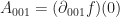
Which is remarkably close to the formula for 1D Taylor series expansions!

Next Time

I will show how to actually implement symmetric tensors in C++11, and give some example applications of multidimensional Taylor series in implicit function modeling and non-linear deformations! I’ll also show how the above expansion can be simplified even further by working in projective coordinates.

Month: August 2011

Multidimensional Taylor Series and Symmetric Tensors