Large voxel terrains may contain millions of polygons. Rendering such terrains at a uniform scale is both inefficient and can lead to aliasing of distant objects. As a result, many game engines choose to implement some form of level of detail based rendering, so that distant terrain is rendered with less geometry.
In this post, I’ll talk about a simple technique based on vertex clustering with some optimizations to improve seam handling. The specific ideas in this article are applied to Minecraft-like blocky terrain using the same clustering/sorting scheme as POP buffers.
Progressively Ordered Primitive (POP) buffers are a special case of vertex clustering, where for each level of detail we round the vertices down to the previous power of two. The cool thing about them is that unlike other level of detail methods, they are implicit, which means that we don’t have to store multiple meshes for each level detail on the GPU.
When any two vertices of a cell are rounded to the same point (in other words, an edge collapse), then we delete that cell from that level of detail. This can be illustrated in the following diagram:
Suppose that each vertex has integer coordinates. Define,
Each of the sets represents the topology mesh at some level of detail, with being the finest, full detail mesh and the coarsest. To get the actual geometry at level , we can take any and compute,
Using this property, we can encode the different levels of detail by sorting the primitives of the mesh from coarse-to-fine and storing a table of offsets:
To render the mesh at any level of detail we can adjust the vertex count, and round the vertices in the shader.
Building POP buffers
To construct the POP buffer, we need to sort the quads and count how many quads are in each LOD. This is an ideal place to use counting sort, which we can do in-place in O(n) time, illustrated in the following psuedo-code:
// Assume MAX_LOD is the total number of levels of detail
// quadLOD(...) computes the level of detail for a quad
function sortByLOD (quads) {
    const buckets = (new Array(MAX_LOD)).fill(0)
    // count number of quads in each LOD
    for (let i = 0; i < quads.length; ++i) {
        buckets[quadLOD(quads[i])] += 1
    }
    // compute prefix sum
    let t = 0;
    for (let i = 0; i < MAX_LOD; ++i) {
       const b = buckets[i]
       buckets[i] = t
       t += b
    }
    // partition quads across each LOD
    for (let i = quads.length - 1; i >= 0; --i) {
        while (true) {
            const q = quads[i]
            const lod = quadLOD(q)
            const ptr = buckets[lod]
            if (i < ptr) {
                break;
            }
            quads[i] = quads[ptr]
            quads[ptr] = q
            buckets[lod] += 1
        }
    }
    // buckets now contains the prefixes for each LOD
    return buckets
}
The quadLOD() helper function returns the coarsest level of detail where a quad is non-degenerate. If each quad is an integer unit square (i.e. not the output from a greedy mesh), then we can take the smallest corner and compute the quad LOD in constant time using a call to count-trailing zeroes. For general quads, the situation is a bit more involved.
LOD computation
For a general axis-aligned quad, we can compute the level of detail by taking the minimum level of detail along each axis. So it then suffices to consider the case of one interval, where the level of detail can be computed by brute force using the following algorithm:
function intervalLOD (lo, hi) {
    for (let i = 0; i <= 32; ++i) {
        if ((lo >> i) === (hi >> i)) {
            return i
        }
    }
}
We can simplify this if our platform supports a fast count-leading-zeroes operation:
function intervalLOD (lo, hi) {
    return countLeadingZeroes(lo ^ hi)
}
Squashed faces
The last thing to consider is that when we are collapsing faces we can end up with over drawing due to rounding multiple faces to the same level. We can remove these squashed faces by doing one final pass over the face array and moving these squashed faces up to the next level of detail. This step is not required but can improve performance if the rendering is fragment processing limited.
Geomorphing, seams and stable rounding
In a voxel engine we need to handle level of detail transitions between adjacent chunks. Transitions occur when we switch from one level of detail to another abruptly, giving a discontinuity. These can edges be hidden using skirts or transition seams at the expense of greater implementation complexity or increased drawing overhead.
In POP buffers, we can avoid the discontinuity by making the level of detail transition continuous, similar to 2D terrain techniques like ClipMaps or CLOD. Observe that we can interpolate between two levels of detail using vertex morphing,
In the original POP buffer paper, they proposed a simple logarithmic model for selecting the LOD parameter as a function of the vertex coordinate :
Where is a bias parameter (based on the display resolution, FOV and hardware requirements) and viewDist is a function that computes the distance to the vertex from the camera. Unfortunately, this LOD function is discontinuous across gaps due to rounding.
The authors of the original POP buffer paper proposed modifying their algorithm to place vertices along the boundary at the lowest level of detail. This removes any cracks in the geometry, but increases LOD generation time and the size of the geometry.
Instead we can solve this problem using a stable version of LOD rounding. Let be the maximum LOD value for the chunk and all its neighbors. Then we compute a fixed point for :
In practice 2-3 iterations is usually sufficient to get a stable solution for most vertices. This iteration can be implemented in a vertex shader and unrolled, giving a fast seamless level of detail selection.
As an aside, this construction seems fairly generic. The moral of the story is really that if we have geomorphing, then we don’t need to implement seams or skirts to get crack-free LOD.
World space texture coordinates
Finally, the last issue we need to think about are texture coordinates. We can reuse the same texturing idea from greedy meshing. For more info see the previous post.
Been a long time since I’ve written anything here. Lately I’ve been working on a new multiplayer WebGL voxel engine for codemao (an educational platform to teach kids programming via games). It’s not live yet, but a bunch of neat ideas have come out of this project. In this post I want to talk about the lighting model and share some of the tricks which were used to speed up processing.
Conceptually the basic lighting system is similar to the one used in Minecraft and Seed of Andromeda with a few small tweaks. For background information, I would recommend the following sources:
This post describes some extensions and optimizations to the basic flood fill lighting model proposed by Ben Arnold. In particular, we show how to adapt ambient occlusion to track a moving sun, and how to improve flood fill performance using word-level parallelism bit tricks.
Recap of flood fill lighting
Flood fill lighting is an approximation of ambient occlusion where lighting values are propagated using a breadth-first search along the 6-faces of each cube. To the best of my knowledge, Minecraft is the first game to use technique to approximate global illumination, but Ben Arnold is the first to write about it in detail. Minecraft tracks two separate lighting channels. One for global light values based on time of day, and one for block light levels derived from objects like torches. This allows for the color of the day light to change dynamically without requiring large terrain updates. Ben Arnold improves on this basic pattern by storing a separate light level for the red/green/blue allowing for colored light sources:
Minecraft: 1 byte = 4 bits for torch light + 4 bits for sky light
Seed of andromeda: 2 bytes = 4 bits red + 4 bits green + 4 bits blue + 4 bits sky
This post: 4 bytes = 4 bits red + 4 bits green + 4 bits blue + 5 * 4 bits sky
Multidirectional sun light
The first improvement we propose in this model is modifying the sky light to support multiple directions. Instead of sampling only sunlight propagation along the y-axis, we also sample along the +/-x axes and the 45-degree diagonal x-y lines and compute ambient contributions for these angle independently:
This requires storing 4 extra light coefficients per-voxel, and if we use 4-bits per coefficient, then this is a total of 16 extra bits. Combined with the previous 16-bits, this means we need 32-bits of extra lighting data per voxel.
To track the lighting values for the other axes we do essentially the same thing for each extra component. In the case of the +/-x axes, it should be clear enough how this works. For the diagonal axes we can trace through a sheared volume. To index into the diagonal textures we take either the sum/ difference of the x and y components and to get the distance along the ray we can just use the y-value.
Word level parallelism
When propagating light field, we need to often perform component-wise operations on the channels of each light field, which we can pack into a single machine word. Here’s a picture of how this looks assuming 4-bits per channel for the simpler case of a 32-bit value:
We could do operations on each channel using bit masking/shifting and looping, however there is a better way: word level parallelism. We’ll use a general pattern of splitting the coefficients in half and masking out the even/odd components separately so we have some extra space to work. This can be done by bit-wise &’ing with the mask 0xf0f0f0f:
Less than
The first operation we’ll consider is a pair-wise less than operation. We want to compare two sets of lighting values and determine which components are < the other. In pseudo-JS we might implement this operation in the following naive way:
function lightLessThan (a, b) {
 let r = 0;
 for (let i = 0; i < 8; ++i) {
   if ((a & (0xf << i)) < (b & (0xf << i))) {
     r |= 0xf << i;
   }
 }
 return r;
}
We can avoid this unnecessary looping using word-level parallelism. The basic idea is to subtract each component and use the carry flag to check if the difference of each component is negative. To prevent underflow we can bitwise-or in a guard so that the carry bits are localized to each component. Here’s a diagram showing how this works:
Putting it all together we get the following psuedo-code:
Building on this we can find component-wise maximum of two light vectors (necessary when we are propagating light values). This key idea is to use the in place bit-swap trick from the identity:
Combined with the above, we can write component-wise max as:
function wlpMax (a, b) {
 return a ^ ((a ^ b) & wlpLT(a, b));
}
Decrement-and-saturate
Finally, in flood fill lighting the light level of each voxel decreases by 1 as we propagate. We can implement a component-wise-decrement and saturate again using the same idea:
function wlpDecHalf (x) {
 // compute component-wise decrement
 const d = ((x & 0xf0f0f0f) | 0x20202020) - 0x1010101;

// check for underflow
 const b = d & 0x10101010;

// saturate underflowed values
 return (d + (b >> 4)) & 0x0f0f0f0f;
}

// decrement then saturate each 4 bit component of x
function wlpDec (x) {
 return wlpDecHalf(x) | (wlpDecHalf(x >> 4) << 4);
}
Previously in this series we covered the basics of collision detection and discussed some different approaches to finding intersections in sets of boxes:
Today, we’ll see how well this theory squares with reality and put as many algorithms as we can find to the test. For those who want to follow along with some code, here is a link to the accompanying GitHub repo for this article:
To get a survey of the different ways people solve this problem in practice, I searched GitHub, Google and npm, and also took several polls via IRC and twitter. I hope that I managed to cover most of the popular libraries, but if there is anything here that I missed, please leave a comment and let me know.
While it is not an objective measurement, I have also tried to document my subjective experiences working each library in this benchmark. In terms of effort, some libraries took far less time to install and configure than others. I also took notes on libraries which I considered, but rejected for various reasons. These generally could be lumped into 3 categories:
Broken: The library did not report correct results.
Too much work: Setting up the library took too long. I was not as rigorous with enforcing a tight bound here, as I tended to give more generous effort to libraries which were popular or well documented. Libraries with 0 stars and no README I generally skipped over.
Irrelevant: While the library may have at first looked like it was relevant, closer inspection revealed that it did not actually solve the problem of box intersection. This usually happened because the library had a suspicious name, or because it was some framework whose domain appeared to include this problem.
A word on JavaScript
For the purpose of this benchmark, I limited myself to consider only JavaScript libraries. One major benefit of JavaScript is that it is easier to install and configure JavaScript libraries, which greatly simplifies the task of comparing a large number of systems. Also, due to the ubiquity of JavaScript, it is easy for anyone to replicate these results or rerun these benchmarks on their own machine. The disadvantage though is that there are not as many mature geometry processing libraries for JavaScript as there are for older languages like C++ or Java. Still, JS is popular enough that I had no trouble finding plenty of things to test although the quality of these modules turned out to be wildly varying.
Implementations surveyed
Brute force
As a control I implemented a simple brute force algorithm in the obvious way. While it is not efficient for large problem sizes, it performs pretty well up to few hundred points.
Bounding volume hierarchy modules
I found many modules implementing bounding volume hierarchies, usually in the form of R-trees. Here is a short summary of the ones which I tested:
rbush: This is one of the fastest libraries for box intersection detection. It also has a very simple API, though it did take a bit of time tuning the branching factor to get best performance on my machine. I highly recommend checking this one out!
rtree: An older rtree module, which appears to have largely been replaced by rbush. It has more features, is more complicated, and runs a bit slower. Still pretty easy to use though.
jsts-strtree: The jsts library is a JavaScript port of the Java Topology Suite. Many of the core implementations are solid, but the interfaces are not efficient. For example, they use the visitor pattern instead of just passing a closure to enumerate objects which requires lots of extra boilerplate. Overall found it clumsy to use, but reasonably performant.
lazykdtree: I included this library because it was relatively easy to set up, even though it ended up being very slow. Also notable for working in any dimension.
Quad trees
Because of their popularity, I decided to make a special section for quad trees. By a survey of modules on npm/GitHub, I would estimate that quad trees are one of the most commonly implemented data structures in JavaScript. However it is not clear to me how much of this effort is serious. After much searching, I was only able to find a small handful of libraries that correctly implemented quad trees based rectangle stabbing:
simple-quadtree: Simple interface, but sluggish performance.
jsts-quadtree: Similar problems as jsts-strtree. Unlike strtree, also requires you to filter out the boxes by further pruning them against your query window. I do not know why it does this, but at least the behavior is well documented.
Beyond this, there many other libraries which I investigated and rejected for various reasons. Here is a (non-exhaustive) list of some libraries that didn’t make the cut:
Google’s Closure Library: This library implements something called “quadtree”, but it doesn’t support any queries other than set membership. I am still not sure what the point of this data structure is.
generic-quadtree: Only implements point-in-rectangle queries, not rectangle-rectangle (stabbing) queries.
quadtree: I’m don’t know what this module does, but it is definitely not a quad tree.
Physics engines
Unfortunately, many of the most mature and robust collision detection codes for JavaScript are not available as independent modules. Instead, they come bundled as part of some larger “physics framework” which implements multiple algorithms and a number of other features (like a scene graph, constraint solver, integrator, etc.). This makes it difficult to extract just the collision detection component and apply it to other problems. Still, in the interest of being comprehensive, I was able to get a couple of these engines working within the benchmark:
p2.js: A popular 2D physics engine written from the ground up in JavaScript. Supports brute force, sweep and prune and grid based collision detection. If you are looking for a good 2D physics engine, check this one out!
Box2D: Probably the de-facto 2D physics engine, has been extremely influential in realtime physics and game development. Unfortunately, the quality of the JS translations are much lower than the original C version. Supports sweep-and-prune and brute force for broad phase collision detection.
oimo.js: This 3D physics engine is very popular in the THREE.js community. It implements brute force, sweep and prune and bounding volume hierarchies for collision detection. Its API is also very large and makes heavy use of object-oriented programming, which comes with some performance tradeoffs. However oimo does deserve credit for being one of the few libraries to tackle 3D collision detection in JavaScript.
I also considered the following physics engines, but ended up rejecting them for various reasons:
cannon.js: To its credit, cannon.js has a very clear API and well documented code. It is also by the same author as p2.js, so it is probably good. However, it uses spheres for broad phase collision detection, not boxes, and so it is not eligible for this test.
GoblinPhysics: Still at very early stages. Right now only supports brute force collision detection, but it seems to be progressing quickly. Probably good to keep an eye on this one.
PhysicsJS: I found this framework incredibly difficult to deal with. I wasted 2 days trying to get it to work before eventually giving up. The scant API documentation was inconsistent and incomplete. Also, it did not want to play nice in node.js or with any other library in the browser, hooking event handlers into all nooks and crannies of the DOM, effectively making it impossible to run as a standalone program for benchmarking purposes. Working with PhysicsJS made me upset.
Matter.js: After the fight with PhysicsJS, I didn’t have much patience for dealing with large broken libraries. Matter.js seems to have many of the same problems, again trying to patch a bunch of weird stuff onto the window/DOM on load, though at least the documentation is better. I spent about an hour with it before giving up.
ammo.js/physijs: This is an emscripten generated port of the popular bullet library, however due to the translation process the API is quite mangled. I couldn’t figure out how to access any of the collision detection methods or make it work in node, so I decided to pass on it.
Range-trees
Finally, I tried to find an implementation of segment tree based intersection for JavaScript, but searching turned up nothing. As far as I know, the only widely used implementation of these techniques is contained in CGAL, which comes with some licensing restrictions and also only works in C++. As a result, I decided to implement of Edelsbrunner & Zomorodian’s algorithm for streaming segment trees myself. You can find the implementation here:
The code is available under a liberal MIT license and easily installable via npm. It should work in any modern CommonJS environment including browserify, iojs and node.js.
Testing procedure
In each of these experiments, a set of boxes was generated, and then sent to each library to compute a checksum of the set of pairs of intersections. Because different libraries expect their inputs in different formats, as a preprocessing step the boxes are converted into whatever data type is expected by the library. This conversion step is not counted towards the total running time. Note that the preparation phase does not include any time required to build associated data structures like search trees or grids; these timings are counted toward the total run time.
Because algorithms for collision detection are output sensitive, care was taken to ensure that the total number of intersections in each distribution is at most , in order to avoid measuring the reporting time for each method.
A limitation of this protocol is that it favors batched algorithms (as would be typically required in CAD applications), and so it may unfairly penalize iterative algorithms like those used in many physics engines. To assess the performance of algorithms in the context of dynamic boxes more work would be needed.
Results
Here is a summary of the results from this benchmark. For a more in depth analysis of the data, please see the associated GitHub repo. All figures in this work were made with plot.ly, click on any of the images to get an interactive version.
Uniform distribution
I began this study by testing each algorithm against the uniform distribution. To ensure that the number of intersections is at most , I borrowed a trick from Edelsbrunner and Zomorodian; and scaled the side length of each box to be while constraining the boxes to remain within the unit hypercube, . A typical sample from this distribution looks like this,
Uniformly distributed boxes
To save time, I split the trials into phases ordered by number of boxes; algorithms which performed took too long on smaller instances were not tested on larger problem sizes. One of the first and most shocking results was a test instance I ran with just 500 boxes:
Here two libraries stand out for their incredibly bad performance: Box2D and lazykdtree. I am not sure why this situation is so bad, since I believe the C version of Box2D does not have these problems (though I need to verify this). Scaling out to 1500 boxes without these two libraries gives the following results:
The next two worst performing libraries were simple-quadtree and rtree. simple-quadtree appears to have worse than quadratic growth, suggesting fundamental algorithmic flaws. rtree’s growth is closer to , but due to the constants involved is still far too slow. As it took too long and there were 2 other representatives of the r-tree data structure in the benchmark, I decided to drop it from larger tests. Moving on to 10k boxes,
At this point, the performance of brute force begins to grow too large, and so it was omitted from the large brute force tests.
Because p2’s sweep method uses an insertion sort, it takes time with a cold start. This causes it to perform close to brute force in almost all cases which were considered. I suspect that the results would be better if p2 was used from a warm start or in a dynamic environment.
Both of jsts’ data structures continue to trend at about growth, however because the constants involved are so large they were also dropped from the large problem size.
10000 boxes appears to be the cut off for real time simulation (or 60fps) at least on my machine. Beyond, this point, even the fastest collision detection algorithm (in this case box-intersect) takes at least 16ms. It is unlikely that any purely JavaScript collision detection library would be able to handle significantly more boxes than this, barring substantial improvements in either CPU hardware or VM technology.
One surprise is that within this regime, box-intersect is consistently 25-50% faster than p2-grid, even though one would expect the complexity of the grid algorithm to beat the time of box-intersect. An explanation for this phenomenon would be that box-intersect enjoys better cache locality (scaling linearly with block size), while hashing causes indirect main memory accesses for each box. If the size of a cache line is , then the cross over point should occur when in 2D. This is illustrated in the following chart which carries out the experiment to 250k boxes,
As expected, somewhere between 10000 and 20000 boxes, p2-grid finally surpasses box-intersect. This is expected as grids realize complexity for uniform distributions, which is ultimately faster than for sufficiently large .
The complexity of rbush on this distribution is more subtle. For the bulk insertion method, rbush uses the “overlap minimizing tree” (OMT) heuristic of Lee and Lee,
The OMT heuristic partitions the space into an adaptive grid at each level of the tree along the quantiles. In the case of a uniform distribution of boxes, this reduces to uniform grid giving a query time of , which for finite gives means that rbush will find all intersections in time. As a result, we can expect that once , rbush-bulk should eventually surpass box-intersect in performance (though this did not occur in my benchmarks). This also suggests another way to interpret the OMT heuristic: it is basically a hedged version of the uniform grid. While not quite as fast in the uniform case, it is more adaptive to sparse data.
Sphere
Of course realistic data is hardly ever uniformly distributed. In CAD applications, most boxes tend to be concentrated in a lower dimensional sub-manifold, typically on the boundary of some region. As an example of this case, we consider boxes which are distributed over the surface of a sphere (again with the side lengths scaled to ensure that the expected number of collisions remains at most ).
A collection of boxes distributed over the boundary of ball.
To streamline these benchmarks, I excluded some of the worst performing libraries from the comparison. Starting with a small case, here are the results:
Again, brute force and p2’s sweep reach similar performance.
More significantly, p2-grid did not perform as well as in the uniform case, running an order of magnitude slower. This is as theory would predict, so no real surprises. Continuing the trend out to 50k boxes gives the following results,
Both p2-grid and jsts-quadtree diverge towards , as grid based partitioning fails for sparse data.
Both rbush and jsts-strtree show similar growth rates, as they implement nearly identical algorithms, however the constant factors in rbush are much better. The large gap in their performance can probably be explained by the fact that jsts uses Java style object oriented programming which does not translate to JavaScript well.
One way to understand the OMT heuristic in rbush, is that it is something like a grid, only hedged against sparse cases (like this circle). In the case of a uniform distribution, it is not quite as fast as a grid, suffering a penalty, while adding robustness against sparse data.
Again box-intersect delivers consistent performance, as predicted.
High aspect ratio
Finally, we come to the challenging case of high aspect ratio boxes. Here we generate boxes which are uniformly distributed in and and stretched along the -axis by a factor of :
A set of boxes with a high aspect ratio
High aspect ratio boxes absolutely destroy the performance of grids and quad trees, causing exponential divergence in complexity based on the aspect ratio. Here are some results,
Even for very small , grids take almost a second to process all intersections for just 10000 boxes. This number can be made arbitrarily high by choosing as extreme an aspect ratio as one likes. Here I select an aspect ratio of , forcing the asymptotic growth of both jsts-quadtree and p2-grid to be . If I had selected the aspect ratio as or , then it would have been possible to increase their running times to some arbitrarily large value. In this benchmark, rbush also grows though by a much slower . Continuing out to 100k boxes, eventually rbush also fails,
In this case rbush-bulk takes more than 40x slower and rbush-bulk more than 70x. Unlike in the case of grids however, these numbers are only realized by scaling in the number of boxes and so they cannot be made arbitrarily large. However, it does illustrate that for certain inputs rbush will fail catastrophically. box-intersect again continues to grow very slowly.
3D
The only libraries which I found that implemented 3D box intersection detection were lazykdtree and oimo.js. As it is very popular, I decided to test out oimo’s implementation on a few small problem sizes. Results like the following are typical:
For large, uniform distributions of boxes, grids are still the best. For everything else, use segment trees.
Brute force is a good idea up to maybe 500 boxes or so.
Grids succeed spectacularly for large, uniform distributions, but fail catastrophically for anything more structured.
Quad trees (at least when properly implemented) realize similar performance as grids. While not as fast for uniform data, they are slightly hedged against boxes of wildly variable size.
RTrees with a tuned heuristic can give good performance in many practical cases, but due to theoretical limitations (see the previous post), they will always fail catastrophically in at least some cases, typically when dealing with boxes having a high aspect ratio.
Zomorodian & Edelsbrunner’s streaming segment tree algorithm gives robust worst case performance no matter what type of input you throw at it. It is even faster than grids for uniform distributions at small problem sizes(<10k) due to superior cache performance.
Overall, streaming segment trees are probably the safest option to select as they are fastest in almost every case. The one exception is if you have a large number of uniformly sized boxes, in which case you might consider using a grid.
Last time, we discussed collision detection in general and surveyed some techniques for narrow phase collision detection. In this article we will go into more detail on broad phase collision detection for closedaxis-aligned boxes. This was a big problem in the 1970’s and early 1980’s in VLSI design, which resulted in many efficient algorithms and data structures being developed around that period. Here we survey some approaches to this problem and review a few theoretical results.
Boxes
A box is a cartesian product of intervals, so if we want to represent a d-dimensional box, it is enough to represent a tuple of d 1-dimensional intervals. There are at least two ways to do this:
As a point with a length
As a pair of upper and lower bounds
For example, in 2D the first form is equivalent to representing a box as a corner point together with its width and height (e.g. left, top, width, height), while the second is equivalent to storing a pair of bounds (e.g. ).
A 2D box is the cartesian product of two 1D intervals.
To test if a pair of boxes intersect, it is enough to check that their projections onto each coordinate axes intersects. This reduces the d-dimensional problem of box intersection testing to the 1D problem of detecting interval overlap. Again, there are multiple ways to do this depending on how the intervals are represented:
Given two intervals represented by their center point and radius, ,
Given two intervals represented by upper and lower bounds, ,
In the first predicate, we require two addition operations, one absolute value and one comparison, while the second form just uses two comparisons. Which version you prefer depends on your application:
In my experiments, I found that the first test was about 30-40% faster in Chrome 39 on my MacBook, (though this is probably compiler and architecture dependent so take it with a grain of salt).
The second test is more robust as it does not require any arithmetic operations. This means that it cannot fail due to overflow or rounding errors, making it more suitable for floating point inputs or applications where exact results are necessary. It also works with unbounded (infinite) intervals, which is useful in many problems.
For applications like games where speed is of the utmost importance, one could make a case for using the first form. However, in applications where it is more important to get correct results (and not crash!) robustness is a higher priority. As a result, we will generally prefer to use the second form.
1D interval intersection
Before dealing with the general case of box intersections in d-dimensions, it is instructive to look at what happens in 1D. In the 1D case, there is an efficient sweep line algorithm to report all intersections. The general idea is to process the end points of each interval in order, keeping track of all the intervals which are currently active. When we reach the start of a new interval, we report intersections with all currently active intervals and it to the active set, and when we reach the end of an interval we delete the interval from the active set:
Finding all intersections in a set of intervals in 1D
If the number of intervals is , then there are events total, and so sorting them all takes time. Processing event requires a scan through the active set, however for each iteration one intersecting pair is reported. If the total number of collisions is , then the amortized cost of looping over the events is . Therefore, the total running time of this algorithm is in .
Sweep and prune
Sweeping is probably the best solution for finding interval overlaps in 1D. The challenge is to generalize this to higher dimensions somehow. One approach is to just run the 1D interval sweep to filter out collisions along some axis, and then use a brute force test to filter these pairs down to an exact set,
The sweep and prune method for box intersection detection.
In JavaScript, here is an illustration of how it could be implemented in terms of the previous 1D sweep algorithm:
//Assume each box is represented by a list of d intervals
//Each interval is of the form [lo,hi]
function sweepAndPrune(boxes) {
  return sweepIntervals(boxes.map(function(box) {
    return box[0]
  }).filter(function(pair) {
    var A = boxes[pair[0]], B = boxes[pair[1]]
    for(var i=1; i<A.length; ++i) {
      if(B[i][1] < A[i][1] || A[i][1] < B[i][0])
        return false
    }
    return true
  })
}
The germ of this idea is contained in Shamos and Hoey’s famous paper on geometric intersection problems,
In the case of rectangles in the plane, one can store the active set in an interval tree (more on this later), giving an optimal algorithm for planar intersection of rectangles. If we just store the active set as an array, then this technique is known as sweep-and-prune collision detection, which is widely used in packages like I-COLLIDE,
For objects which are well separated along some axis, the simple sweep-and-prune technique is very effective at speeding up collision detection. However, if the objects are grouped together, then sweep-and-prune is less effective, realizing a complexity no better than brute force .
Uniform grids
After brute force, grids are one of the simplest techniques for box intersection detection. While grids have been rediscovered many times, it seems that Franklin was one of the first to write extensively about their use in collision detection,
Today, grids are used for many different problems, from small video games all the way up to enormous physical simulations with millions of bodies. The grid algorithm for collision detection proceeds in two phases; first we subdivide space into uniformly sized cubes of side length , then insert each of the boxes into the cells they overlap. Boxes which share a common grid cell are tested for overlaps:
In a grid, boxes are inserted into cells which they overlap incrementally, and tested against other boxes in the same grid cells.
Implementing a grid for collision detection is only just more complicated than sweep and prune:
//Same convention as above, boxes are list of d intervals
// H is the side length for the grid
function gridIntersect2D(boxes, H) {
  var grid = {}, result = [], x = [0,0]
  boxes.forEach(function(b, id) {
    for(x[0]=Math.floor(b[0][0]/H); x[0]<=Math.ceil(b[0][1]/H); ++x[0])
    for(x[1]=Math.floor(b[1][0]/H); x[1]<=Math.ceil(b[1][1]/H); ++x[1]) {
      var list = grid[x]
      if(list) {
        list.forEach(function(otherId) {
          var a = boxes[otherId]
          for(var i=0; i<2; ++i) {
            var s = Math.max(a[i][0], b[i][0]),
                t = Math.min(a[i][1], b[i][1])
            if(t < s || Math.floor(s/H) !== x[i])
              return
          }
          result.push([id, otherId])
        })
        list.push(id)
      } else grid[x] = [id]
    }
  })
  return result
}
Note here how duplicate pairs are handled: Because in a grid it is possible that we may end up testing the same pair of boxes against each other many times, we need to be careful that we don’t accidentally report multiple pairs of collisions. One way to prevent this is to check if the current grid cell is the lexicographically smallest cell in their intersection. If it isn’t, then we skip reporting the pair.
While the basic idea of a grid is quite simple, the details of building efficient implementations are an ongoing topic of research. Most implementations of grids differ primarily in how they manage the storage of the grid itself. There are 3 basic approaches:
Dense array: Here the grid is encoded as a flat array of memory. While this can be expensive, for systems with a bounded domain and a dense distribution of objects, the fast access times may make it preferable for small systems or parallel (GPU) simulations.
Hash table: For small systems which are more sparse, or which have unbounded domains, a hash table is generally preferred. Accessing the hash table is still , however because it requires more indirection iterating over the cells covering a box may be slower due to degraded data locality.
Sorted list: Finally, it is possible to skip storing a grid as such and instead store the grid implicitly. Here, each box generates a cover of cells which are then appended to a list which is then sorted. Collisions correspond to duplicate cells which can be detected with a linear scan over the sorted list. This approach is easy to parallelize and has excellent data locality, making it efficient for systems which do not fit in main memory or need to run in parallel. However, sorting is asymptotically slower than hashing, requiring an extra overhead, which may make it less suitable for problems small enough to fit in RAM.
Analyzing the performance of a grid is somewhat tricky. Ultimately, the grid algorithm’s complexity depends on the distribution of boxes. At a high level, there are 3 basic behaviors for grids:
Too coarse: If the grid size is too large, then it won’t be effective at pruning out non-intersecting boxes. As a result, the algorithm will effectively degenerate to brute force, running in .
Too fine: An even worse situation is if we pick a grid size that is too small. In the limit where the grid is arbitrarily fine, a box can overlap an infinite number of cells, giving the unbounded worst case performance of !!!
Just right: The best case scenario for the grid is that the objects are uniformly distributed in both space and size. Ideally, we want each box to intersect at most cells and that each cell contains at most objects. In this case, the performance of a grid becomes (using a grid or hash table), or for sorted lists, which for small is effectively an optimal complexity.
Note that these cases are not mutually exclusive, it is possible for a grid to be both too sparse and too fine at the same time. As a result, there are inputs where grids will always fail, no matter what size you pick. These difficulties can arise in two situations:
Size variation: If the side lengths of the boxes have enormous variability, then we can’t pick just one grid size. Hierarchical grids or quad trees are a possible solution here, though it remains difficult to tune parameters like the number of levels.
High aspect ratio: If the ratio of the largest to smallest side of the boxes in the grid is too extreme, then grids will always fail catastrophically. There is no easy fix or known strategy to avoid this failure mode other than to not use a grid.
While this might sound pessimistic, it is important to remember that when grids work they are effectively optimal. The trouble is that when they fail, it is catastrophic. The bottom line is that you should use them only if you know the distribution of objects will be close to uniform in advance.
Partition based data structures
After grids, the second most widely recommended approach to collision detection are partition based tree data structures. Sometimes called “bounding volume hierarchies,” partition based data structures recursively split space into smaller regions using trees. Objects are iteratively tested against these trees, and then inserted into the resulting data structure.
Bounding volume hierarchy intersection proceeds by recursively inserting rectangles into the root of the tree and expanding subtrees.
In psuedo-JavaScript, here is how this algorithm works:
function bvhIntersect(boxes) {
  var tree = createEmptyTree(), result = []
  boxes.forEach(function(box, id) {
    bvhQuery(tree, box).forEach(function(otherBox) {
      result.push([box, otherBox])
    })
    bvhInsert(tree, box)
  })
  return result
}
While the insertion procedure is different for each tree-like data structure, in bounding volume hierarchies querying always follows the same general pattern: starting from the root of the tree, recursively test if any children intersect the object. If so, then visit those children, continuing until the leaves of the tree are reached. Again, in psuedo-JavaScript:
The precise complexity of this meta-algorithm depends on the structure of the tree, the distribution of the boxes and how insertion is implemented. In the literature, there are many different types of bounding volume hierarchies, which are conventionally classified based on the shape of the partitions they use. Some common examples include:
Within each of these general types of trees, further classification is possible based on the partition selection strategy and insertion algorithm. One of the most comprehensive resources on such data structures is Samet’s book,
It would seem like the above description is too vague to extract any meaningful sort of analysis. However, it turns out that using only a few modest assumptions we can prove a reasonable lower bound on the worst case complexity of bvhIntersect. Specifically, we will require that:
The size of a tree with items is at most bits.
Each node of the tree is of bounded size and implemented using pointers/references. (As would be common in Java for example).
Querying the tree take time, where is the number of items in the tree.
In the case of all the aforementioned trees these conditions hold. Furthermore, let us assume that insertion into the tree is “cheap”, that is at most polylogarithmic time; then the total complexity of bvhIntersect is in the worst case,
.
Now here is the trick: using the fact that the trees are all made out of a linear number of constant sized objects, we can bound the complexity of querying by a famous result due to Chazelle,
More specifically, he proved the following theorem:
Theorem: If a data structure answers box intersection queries in time, then it uses at least bits.
As a corollary of this result, any (reasonable) bounding volume hierarchy takes at least time per query. Therefore, the worst case time complexity of bvhIntersect is slower than,
.
Now this bound does come with a few caveats. Specifically, we assumed that the query overhead was linear in the number of reported results and neglected interactions with insertion. If is practically , then it is at least theoretically possible to do better. Again, we cite a result due to Chazelle, which shows that it is possible to report rectangle intersection queries in time using space,
Finally, let us look at one particular type of bounding volume hierarchy in detail; specifically the R-tree. Originally invented by Guttmann, R-trees have become widely used in GIS databases due to their low storage overhead and ease of implementation,
The high level idea behind an R-tree is to group objects together into bounding rectangles of increasing size. In the original paper, Guttmann gave several heuristics for construction and experimentally validated them. Agarwal et al. showed that the worst case query time for an R-tree is and gave a construction which effectively matches this bound,
Disappointingly, this means that in the worst case using R-trees as a bounding volume hierarchy gives an overall time complexity that is only slightly better than quadratic. For example in 2D, we get , and for 3D .
Still, R-trees are quite successful in practice. This is because for cases with smaller query rectangles the overhead of searching in an R-tree approaches . Situations where the complexity degenerates to tend to be rare, and in practice applications can be designed to avoid them. Moreover, because R-trees have small space overhead and support fast updates, they are relatively cheap to maintain as an index. This has lead to them being used in many GIS applications, where the problem sizes make conserving memory the highest priority.
Range tree based algorithms
So far none of the approaches we’ve seen have managed to break the barrier in the worst case (with the exception of 1D interval sweeping and a brief digression into Shamos & Hoey’s algorithm). To the best of my knowledge, all efficient approaches to this problem make some essential use of range trees. Range trees were invented by Bentley in 1979, and they solve the orthogonal range query problem for points in time using space (these results can be improved somewhat using fractional cascading and other more sophisticated techniques). The first application of range tree like ideas to rectangle intersections was done by Bentley and Wood,
In this paper they, introduced the concept of a segment tree, which solves the problem of interval stabbing queries. One can improve the space complexity of their result in 2D using an interval tree instead, giving a algorithm for detecting rectangle intersections. These results were generalized to higher dimensions and improved by Edelsbrunner in a series of papers,
Amongst the ideas in those papers is the reduction of the intersection test to range searching on end points. Specifically, it is true that if two 1D intervals intersect, then at least one of them contains the end points of the other box. The recursive application of this idea allows one to use a range tree to resolve box intersection queries in dimensions using space and time.
Streaming algorithms
The main limitation of range tree based algorithms is that they consume too much space. One way to solve this problem is to use streaming. In a streaming algorithm, the tree is built lazily as needed instead of being constructed in one huge batch. If this is done carefully, then the box intersections can be computed using only extra memory (or even if we allow in place mutation) instead of . This approach is described in the following paper by Zomorodian and Edelsbrunner,
In this paper, the authors build a segment tree using the streaming technique, and apply it to resolve bipartite box interactions. The overall time complexity of the method is , which matches the results for segment trees.
Next time
In the next part of this series we will look at some actual performance data from real benchmarks for each of these approaches. Stay tuned!
Collision, or intersection, detection is an important geometric operation with a large number of applications in graphics, CAD and virtual reality including: map overlay operations, constructive solid geometry, physics simulation, and label placement. It is common to make a distinction between two types of collision detection:
Narrow phase: Test if 2 objects intersect
Broad phase: Find all pairs of intersections in a set of n objects
In this series, I want to focus on the latter (broad phase), though first I want to spend a bit of time surveying the bigger picture and explaining the significance of the problem and some various approaches.
Narrow phase
The approach to narrow phase collision detection that one adopts depends on the types of shapes involved:
Constant complexity shapes
While it is true that for simple shapes (like triangles, boxes or spheres) pairwise intersection detection is a constant time operation, because it is frequently used in realtime applications (like VR, robotics or games) an enormous amount of work has been spent on optimizing. The book “Realtime Collision Detection” by Christer Ericson has a large collection of carefully written subroutines for intersection tests between various shapes which exploit SIMD arithmetic,
For more complicated shapes (that is shapes with a description length longer than ) detecting intersections becomes algorithmically interesting. One important class of objects are convex polytopes, which have the property that between any pair of points in the shape the straight line segment connecting them is also contained in the shape. There are two basic ways to describe a convex polytope:
V-Polytope: As the set of all convex combinations of a finite set of points and possibly infinite direction vectors (aka 1D cones)
These two representations are equivalent in their descriptive power (though proving this is a bit tricky). The process of converting a V-polytope into an H-polytope is called taking the “convex hull” of the points, and the dual algorithm of converting an H-polytope into a V-polytope is called “vertex enumeration.”
The problem of testing if two convex polytopes intersect is a special case of linear programming feasibility. This is pretty easy to see for H-polytopes; suppose that:
Where,
is a n-by-d matrix
is a n-dimensional vector
is a m-by-d matrix
is a m-dimensional vector
Then the region is equivalent to the feasible region of a system of linear inequalities in variables:
If this system has a solution (that is it is feasible), then there is a common point in the interior of both sets which satisfies the above equations. The case for V-polytopes is similar, and leads to a transposed system of variables in constraints (that is, it is the asymmetric dual of the above linear program).
Linear programs are a special case of LP-type problems, and for low dimensions can be solved linear time in the number of half spaces or variables. (For those curious about the details, here are somelectures). For example, using Seidel’s algorithm testing the feasibility of the above system takes time, which for fixed dimension is just . The dependence on can be improved using more advanced techniques like Clarkson’s algorithm.
Preprocessing
If we are willing to preprocess the polytopes, it is possible to do exponentially better than . In 2D, the problem of testing intersection between a pair of polygons reduces to calculating a pair of tangent lines between the polygons. There is a well known algorithm for solving this in time by binary search (assuming that the vertices/faces of the polygon are stored in an ordered array, which is almost always the case).
The 3D case is a bit trickier, but it can be solved in using a more sophisticated data structure,
For interactive applications like physics simulations, another important technique is to reuse previous closest points in calculating distances (similar to using a warm restart in the simplex method for linear programming). This ideas were first applied to collision detection in the now famous Lin-Canny method:
For “temporally coherent” collision tests (that is repeatedly solved problems where the shapes involved do not change much) the complexity of this method is practically constant. However, because it relies on a good initial guess, the performance of the Lin-Canny method can be somewhat poor if the objects move rapidly. More recent techniques like H-walk improve on this idea by combining it with fast data structures for linear programming queries, such as the Dobkin-Kirkpatrick hierarchy to get more robust performance:
Outside of convex polytopes, the situation for resolving narrow phase collisions efficiently and exactly becomes pretty hopeless. For algebraic sets like NURBS or subdivision surfaces, the fastest known methods all reduce to some form of approximate root finding (usually via bisection or Newton’s method). Exact techniques like Grobner basis are typically impractical or prohibitively expensive. In constructive solid geometry working with semialgebraic sets, it is even worse where one must often resort to general nonlinear optimization, or in the most extreme cases fully symbolic Tarski-Seidenberg quantifier elimination (like the cylindrical algebraic decomposition).
Measure theoretic methods
I guess I can say a few words about some of my own small contributions here. An alternative to computing the distance between two shapes for testing separation is to compute the volume of their intersection, . If this volume is , then the shapes collide. One way to compute this volume is to rewrite it as an integral. Let denote the indicator function of , then
This integral is essentially a dot product. If we perform an expansion of in some basis, (for example, as Fourier waves), then we can use that to approximate this volume. If we do this expansion carefully, then with enough work we can show that the resulting approximation preserves something of the original geometry. For more details, here is a paper I wrote:
The advantage to this type of approach to collision detection is that it can support any sort of geometry, no matter how complicated. This is because the cost of the testing intersections scales with the accuracy of the collision test in a predictable, well-defined way. The disadvantage though is that at high accuracies it is slower than other exact techniques. Whether it is worthwhile or not depends on the desired accuracy, the types of shapes involved and if additional information like a separating axis is needed and so on.
Broad phase
Given a fast narrow phase collision test, we can solve the broad phase collision detection problem for objects in calls to the underlying test. As the number of reported collisions could be in the worst case, this would seem optimal. However, we can get a sharper picture using a more detailed output sensitive analysis. To do this, define k to be the number of reported intersections, and let us then analyze the time required to do the collision detection as a function of both n and k. Using output sensitive analysis, there is also a lower bound of (for comparison based algorithms) by reduction to the element uniqueness problem.
Special cases
If we are only allowed to use pairwise intersection tests and know no other property of the shapes, then it is impossible to compute all pairwise intersections any faster than . However, for special types of shapes in low dimensional spaces substantially faster algorithms are known:
Line segments
For line segments in the plane, it is possible to report all intersections in time using a sweep line algorithm. If , this is a big improvement over naive brute force. This technique can also be adapted to compute intersections in sets of general convex polygons by decomposing them into segments, and then building a secondary point location data structure to handle the case where a polygon is completely contained in another.
Uniformly sized and distributed balls
It is also possible to find all intersections in a collection of balls with constant radii in optimal time, assuming that the number of balls any single ball intersects is at most . The key to this idea is to use a grid, or hash table to detect collisions. This process is both simple to implement and has robust performance, and so it is used in many simulations and video games.
Axis aligned boxes
Finally, it is possible to detect all intersections in a collection of axis aligned boxes in time, though we will postpone talking about this until next time.
General objects and bounding volumes
For general objects, no algorithms with running time substantially faster than are known. However, we can in practice still get a big speed up by using a simpler broad phase collision test to filter out intersections. The main idea is to cover each object, , with some simpler shape called a bounding volume. If a pair of bounding volumes do not intersect, then the shapes which they are covering can not intersect either. In this way, bounding volumes can be used to prune down the set of collision tests which must be performed.
In practice, the most common choice for a bounding volume is either a box or a sphere. The reason for this is that boxes and spheres support efficient broad phase intersection tests, and so they are relatively cheap.
Spheres tend to be more useful if all of the shapes are more or less the same size, but computing tight bounding spheres is slightly more expensive. For example, if the objects being intersected consist of uniformly subdivided triangle meshes, then spheres can be a good choice of bounding volume. However, spheres do have some weakness. Because testing sphere intersection requires multiplication, it is harder to do it exactly than it is for boxes. Additionally, for spheres of highly variable sizes it is harder to detect intersections efficiently.
Computing intersections in boxes on the other hand tends to be much cheaper, and it is simpler to exactly detect if a pair of boxes intersect. Also for many shapes boxes tend to give better approximations than spheres, since they can have skewed aspect ratios. Finally, broad phase box intersection has theoretically more robust performance than sphere intersection for highly variable box sizes. Perhaps based on these observations, it seems that most modern high performance physics engines and intersection codes have converged on axis-aligned boxes as the preferred primitive for broad phase collision detection. (See for example, Bullet, Box2D)
Bipartite vs complete
It is sometimes useful to separate objects for collision detection into different groups. For example if we are intersecting water-tight meshes, it is useless to test for self intersections. Or as another example, in a shooter game we only need to test the player’s bullets against all enemies. These are both examples of bipartite collision detection. In bipartite collision detection, we have two groups of objects (conventionally colored red and blue), and the goal is to report all pairs of red and blue objects which intersect.
Range searching and more references
There is a large body of literature on intersection detection and the related problems of range searching. Agarwal and Erickson give an excellent survey of these results in the following paper,
Last time, I finished up talking about latency issues for networked video games. Today I want to move onto the other major network resource, which is bandwidth. Compared to latency, bandwidth is much easier to discuss. This has been observed many times, perhaps most colorfully by Stuart Cheshire:
Though that article is pretty old, many of its points still ring true today. To paraphrase a bit, bandwidth is not as big a deal as latency because:
Analyzing bandwidth requirements is easy, while latency requirements are closely related to human perception and the nature of the game itself.
Bandwidth scales cheaply, while physical constraints impose limitations on latency.
Optimizing for low bandwidth usage is a purely technical problem, while managing high latency requires application specific design tradeoffs.
Costs of bandwidth
But while it is not as tough a problem, optimizing bandwidth is still important for at least three reasons:
Some ISPs implement usage based billing via either traffic billing or download quotas. In this situation, lowering bandwidth reduces the material costs of running the game.
High bandwidth consumption can increase the latency, due to higher probability of packets splitting or being dropped.
Bandwidth is finite, and if a game pushes more data than the network can handle it will drop connections.
The first of these is not universally applicable, especially for small, locally hosted games. In the United States at least, most home internet services do not have download quotas, so optimizing bandwidth below a certain threshold is wasted effort. On the other hand many mobile and cloud based hosting services charge by the byte, and in these situations it can make good financial sense to reduce bandwidth as much as possible.
The second issue is also important, at least up to a point. If updates from the game do not fit within a single MTU, then they will have to be split apart and reassembled. This increases transmission delay, propagation delay, and queuing delay. Again, reducing the size of a state update below the MTU will have no further effect on performance.
It is the third issue though that is the most urgent. If a game generates data at a higher rate than the overall throughput of the connection, then eventually the saturated connection will increase the latency towards infinity. In this situation, the network connection is effectively broken, thus rendering all communication impossible causing players to drop from the game.
Variables affecting bandwidth
Asymptotically the bandwidth consumed by a game is determined by three variables:
= number of players
= frequency of updates
= the size of the game state
In this model, the server needs to send bits/(second * player) or total bits. Clients have a downstream bandwidth of and upstream of just . Assuming a shared environment where every player sees the same state, then . This leaves us with two independent parameters, and , that can be adjusted to reduce bandwidth.
Player caps
The easiest way to conserve bandwidth is to cap the number of players. For small competitive games, like Quake or Starcraft, this is often than sufficient to solve all bandwidth problems. However, in massively multiplayer games, the purpose of bandwidth reduction is really to increase the maximum number of concurrent players.
Latency/bandwidth tradeoffs
Slowing down the update frequency also reduces bandwidth consumption. The cost is that the delay in processing player inputs may increase by up to . Increasing can help reduce lag but only up to a point, beyond which the round trip time dominates.
Some games use a variable update frequency to throttle back when they are under high load. For example, EVE Online does this to maintain stability when many players are clustered within the same zone. They call this technique “time dilation” and explain how it works in a short dev blog:
Decreasing the update frequency causes the game to degrade gracefully rather than face an immediate and catastrophic connection loss due to bandwidth over saturation. We can estimate the amount of time dilation in a region with players, given that that the throughput of the connection is bits/second as,
.
That is the time dilation due to bandwidth constraints should vary as the inverse square of the number of players in some region.
State size reductions
As we just showed, it is always possible to shrink the bandwidth of a game as low as we like by throttling updates or capping the number of players. However, both of these methods weaken the user experience. In this section we consider reductions to the state size itself. These optimizations do not require any sacrifices in gameplay, but are generally more limited in what they can achieve and also more complicated to implement.
Serialization
The most visible target for state bandwidth optimization is message serialization, or marshalling. While it is tempting to try first applying optimization effort to this problem, serialization improvements give at most a constant factor reduction in bandwidth. At the risk of sounding overly judgmental, I assert that serialization is a bike shed issue. Worrying too much about it up front is probably not a wise use of time.
One approach is to adopt some existing serialization protocol. In JavaScript, the easiest way to serialize objects is to use JSON.stringify(). There are also a number of binary equivalent JSON formats, like BSON or MessagePack which can be used interchangeably and save a few bytes here and there. The main drawback to JSON is that serialized objects can’t contain any circular references, and that once they are serialized they will lose all of their function properties and prototypes. As a result, it is easier to use JSON for sending small hierarchically structured messages than process gigantic amorphous interconnected networks of objects. For these latter situations, XML may be more suitable. XML has the advantage that it is extremely flexible, but the disadvantage that it is much more complex.
Both JSON and XML are generic, schema-less serialization formats and so they are limited with respect to the types of optimizations they can perform. For example, if a field in an object is a US phone number then serializing it in JSON takes about 9 bytes in UTF-8. But there are only possible US phone numbers, and so any such number can be encoded in bits, or a little under 4 bytes. In general, given more type information it is possible to achieve smaller encodings.
Google’s Protocol Buffers are an example of a serialization format which uses structured schemas. In the XML world there has been some research into schema based compressors, though they are not widely used. For JSON, there don’t appear to be many options yet, however, there has been some work on creating a standard schema specification for JSON documents.
Compression
Another way to save a bit of space is to just compress all of the data using some standard algorithm like LZMA or gzip. Assuming a streaming communication protocol, like TCP, then this amounts to piping the data through your compressor of choice, and piping the output from that stream down the wire.
In node.js, this is can be implemented with the built in zlib stream libraries, though there are a few subtle details that need to be considered. The first is that by default zlib buffers up to one chunk before sending a write, which adds a lot of extra latency. To fix this, set the Z_PARTIAL_FLUSH option when creating the stream to ensure that packets are serialized in a timely manner. The second and somewhat trickier issue is that zlib will split large packets into multiple chunks, and so the receiver will need to implement some extra logic to combine these packets. Typically this can be done by prefixing each packet with an integer that gives the length of the rest of the message, and then buffering until the transfer is complete.
One draw back to streaming compression is that it does not work with asynchronous messaging or “datagram” protocols like UDP. Because UDP packets can be dropped or shuffled, each message must be compressed independently. Instead, for UDP packets a more pragmatic approach is to use less sophisticated entropy codes like Huffman trees or arithmetic encoding. These methods do not save as much space as zlib, but do not require any synchronization.
Patching
Another closely related idea to compression is the concept of patch based updates. Patching, or diff/merge algorithms use the mutual information between the previously observed states of the game and the transmitted states to reduce the amount of data that is sent. This is more-or-less how git manages commits, which are stored as a sparse set of updates. In video games, patch based replication is sometimes called “delta compression“. The technique was popularized by John Carmack, who used it in Quake 3’s networking code.
Area of interest management
Finally, the most effective way to reduce the size of updates is to replicate fewer objects. That is, given any player we only replicate some subset of the state which is relevant to what the player is currently seeing. Under the right conditions, this asymptotically reduces bandwidth, possibly below . More generally, updates to objects can be prioritized according to some measure of relevance and adaptively tuned to the use available bandwidth.
These techniques are called area of interest management, and they have been researched extensively. At a broad level though, we classify area of interest management strategies into 3 categories:
Rule based: Which use game specific rules to prioritize updates
Static: Which split the game into predefined disjoint zones
Geometric: Which prioritize updates based on the spatial distribution of objects
This is roughly in order of increasing sophistication, with rule based methods being the simplest and geometric algorithms requiring the most analysis.
Rule based methods
Some games naturally enforce area of interest management by the nature of their rules. For example in a strategy game with “fog of war“, players should not be allowed to see hidden objects. Therefore, these objects do not need to be replicated thus saving bandwidth. More generally, some properties of objects like the state of a remote player’s inventory or the AI variables associated to computer controlled opponent do not need to be replicated as well. This fine grained partitioning of the state into network relevant and hidden variables reduces the size of state updates and prevents cheating by snooping on the state of the game.
Static partitioning
Another strategy for managing bandwidth is to partition the game. This can be done at varying levels of granularity, ranging from running many instances of the simulation in parallel to smaller scale region based partitioning. In each region, the number of concurrent players can be capped or the time scale can be throttled to give a bound on the total bandwidth. Many older games, like EverQuest, use this strategy to distribute the overall processing load. One drawback from this approach is that if many players try to enter a popular region, then the benefits of partitioning degrade rapidly. To fix this, modern games use a technique called instancing where parallel versions of the same region are created dynamically to ensure an overall even distribution of players.
Geometric algorithms
Geometric area of interest management prioritizes objects based on their configurations. Some of the simplest methods for doing this use things like the Euclidean distance to the player. More sophisticated techniques take into account situation specific information like the geodesic distance between objects or their visibility. A very accessible survey of these techniques was done by Boulanger et al.:
While locality methods like this are intuitive, distance is not always the best choice for prioritizing updates. In large open worlds, it can often be better to prioritize updates for objects with the greatest visual salience, since discontinuities in the updates of these objects will be most noticeable. This approach was explored in the SiriKata project, which used the projected area of each object to prioritize network replication. A detailed write up is available in Ewen Cheslack-Postava’s dissertation:
Pragmatically, it seems like some mixture of these techniques may be the best option. For large, static objects the area weighted prioritization may be the best solution to avoid visual glitches. However for dynamic, interactive objects the traditional distance based metrics may be more appropriate.
Final thoughts
Hopefully this explains a bit about the what, why and how of bandwidth reduction for networked games. I think that this will be the last post in this series, but probably not the last thing I write about networking.
Last time in this series, I talked about latency and consistency models. I wanted to say more about the last of these, local perception filtering, but ended up running way past the word count I was shooting for. So I decided to split the post and turn that discussion into today’s topic.
Causality
Sharkey and Ryan justified local perception filters based on the limitations of human perception. In this post I will take a more physical approach derived from the causal theory of special relativity. For the sake of simplicity, we will restrict ourselves to games which meet the following criteria:
Many games meet these requirements. For example, in Realm of the Mad God, gameplay takes place in a flat 2D space. Objects like players or projectiles behave as point-masses moving about their center. Interactions only occur when two objects come within a finite distance of each other. And finally, no projectile, player or monster can move arbitrarily fast. The situation is pretty similar for most shooters and MMOs. But not all games fit this mold. As non-examples, consider any game with rigid body dynamics, non-local constraints or instant-hit weapons. While some of the results in this article may generalize to these games, doing so would require a more careful analysis.
Physical concepts
The basis for space-time consistency is the concept of causal precedence. But to say how this works, we need to recall some concepts from physics.
Let be the dimension of space and let denote a dimensional real vector space. In the standard basis we can split any vector into a spatial component and a time coordinate. Now let be the maximum velocity any object can travel (aka the speed of light in the game). Then define an inner product on ,
Using this bilinear form, vectors can be classified into 3 categories:
As a special consideration, we will say that a vector is causalif it is either time-like or null. We will suppose that time proceeds in the direction. In this convention, causal vectors are further classified into 3 subtypes:
Future-directed:
Zero:
Past-directed:
In the same way that a Euclidean is constructed from a normed vector space, space-time is a psuedo-Euclidean space associated to the index-1 vector space and its inner product. We will assume that everyevent (eg collision, player input, etc.) is associated to a unique point in space-time and when it is unambiguous, we will identify the space-time point of the event with itself. Objects in the game are points and their motions sweep out world lines (or trajectories) in space-time.
The relationship between these concepts can be visualized using a Minkowski diagram:
An ordered sequence of events is space-time consistent if for all , .
Space-time consistency is a special case of causal consistency. Relativistic causal precedence is stricter than causality consistency, because it does not account for game specific constraints on interactions between objects. For example, a special effect might not influence any game objects, yet in a relativistic sense it causally precedes all events within its future light cone. Still space-time consistency is more flexible than strict temporal consistency, and as we shall see this can be exploited to reduce latency.
Cone of uncertainty
As a first application of space-time consistency, we derive a set of sufficient conditions for dead-reckoning to correctly predict a remote event. The basis for this analysis is the geometric concept of a light cone, which we now define:
Any closed regular set determines a pair of closed regular sets called its causal future and causal past, respectively:
Causal future:
Causal past:
According to our assumptions about the direction of time, if an event had any causal influence on an event in , then it must be contained in . Conversely, events in can only influence future events in . When the set is a singleton, then is called the future light cone of , and is the past light cone, and the set is the light cone of .
The causal future and past are idempotent operators,
,
.
Sets which are closed under causal past/future are called closed causal sets. If is a closed causal set, then so is its regularized complement,
,
.
Now, to connect this back to dead-reckoning, let us suppose that there are two types of objects within the game:
Active entities: Whose motion is controlled by non-deterministic inputs from a remote machine
Passive entities: Whose trajectory is determined completely by its interactions with other entities.
For every active entity, we track an event which is the point in space-time at which it most recently received an input from its remote controller. Let be the set of all these events. We call the causal future the cone of uncertainty. Events outside the cone of uncertainty are causally determined by past observations, since as we stated above . Consequently, these events can be predicted by dead-reckoning. On the other hand, events inside could possibly be affected by the actions of remote players and therefore they cannot be rendered without using some type of optimistic prediction.
Here is a Minkowski diagram showing the how the cone of uncertainty evolves in a networked game as new remote events are processed:
The cone of uncertainty illustrated. In this Minkowski diagram, the vertical axis represents time. The world lines for each active object are drawn as colored paths. The grey region represents the cone of uncertainty, and is updated as new remote events are processed.
Cauchy surfaces
In this section we consider the problem of turning a -dimensional collection of world lines in space-time into a -dimensional picture of the state of the world. The geometry of this process is encoded by a Cauchy surface. Intuitively, a Cauchy surface captures an instant in space-time as it is perceived by some observer. The rendered state of objects are determined by the points at which their world lines intersect this surface. That these intersections are well-defined motivates the following definition:
A hypersurface is a Cauchy surface if every time-like curve extends to one which intersects exactly once.
This is not the only way to define a Cauchy surface. Equivalently,
Proposition 1: Any Cauchy surface partitions a flat space-time into 3 regions:
The interior of the causal future:
The interior of the causal past:
And itself
If is a maximal set with these properties, then is a Cauchy surface.
In a flat space-time, Cauchy surfaces can be parameterized by spatial coordinates. Let be a Cauchy surface and ,
.
Then,
.
The inverse question of when a function determines a Cauchy surface is answered by the following theorem:
Theorem 1: A function determines a Cauchy surface if and only if the subgradient of is bounded by .
Proof: To show that this condition is sufficient, it is enough to prove that any time parameterized time-like curve intersects the surface only once. To show that the curve crosses at least once, recall proposition 1 implies that partitions into 3 regions, and , and that the curve begins in the causal past of and ends in the causal future, so by the intermediate value theorem the must cross . Now let be a point of intersection between the curve and the surface. Then the entire future of the curve is contained in the open cone . Similarly, because , no other points on intersect . Ditto for all the points in the causal past, and so any intersection must be unique. To show necessity, take any Cauchy surface and construct the field as shown above. Suppose that there is some point and unit vector where . Without loss of generality, assume . Then there exists some where . Construct the time-like curve . By the intermediate value theorem, crosses in two locations and so is not Cauchy. QED
Consistency revisited
Rendering a game amounts to selecting a Cauchy surface and intersecting it with the world lines of all objects on the screen. The spatial coordinates of these intersections are then used to draw objects to the screen. From this perspective one can interpret a consistency model as determining a Cauchy surface. We now apply this insight to the three consistency models which were discussed last time.
Starting with strict consistency, define be the time of the oldest-most recent input from a remote player. Then define a constant Cauchy surface,
.
As we did with the cone of uncertainty, we can visualize the evolution of this Cauchy surface with a Minkowski diagram:
A visualization of the Cauchy surface for strict consistency. The orange line represents the Cauchy surface viewed by the local (red) player. Note that this is some time behind the most recently acknowledged input.
The same analysis applies to optimistic consistency. Let be the time that the most recent local input was processed. Then the optimistic Cauchy surface is,
.
Which gives the following Minkowski diagram:
An optimistic Cauchy surface (shown in orange). The surface tracks the local red player closely, giving more responsive inputs. Unfortunately, the optimistic Cauchy surface intersects the cone of uncertainty and so it requires local prediction to extrapolate the position of remote objects.
Unlike in the case of the strict consistency, the optimistic causal surface intersects the cone of uncertainty. As a result, it requires prediction to extrapolate the state of remote entities.
Finally, here is a Minkowski diagram showing the Cauchy surface of a local perception filter:
The Cauchy surface for a local perception filter. Note that this surface closely follows the local player, yet does not intersect the cone of uncertainty.
Time dilation
Local perception filters make finer geometric tradeoffs between local responsiveness and visual consistency. They achieve this by using a curved Cauchy surface. This has a number of advantages in terms of improving responsiveness, but introduces time dilation as a side effect. In a game, this time dilation will be perceived as a virtual acceleration applied to remote objects. To explain this concept, we need to make a distinction between local time and coordinate time. Coordinate time, , is the time component of the coordinates of an event in Minkowski space-time. Local time, , is the time that an event is rendered for a local user.
Now suppose that we have a Cauchy surface, varying as function of local time. We want to compute the time dilation experienced by an object with a coordinate time parameterized world line, . In this situation, define the mapping , that relates local time to the particle’s coordinate time,
.
The time dilation observed in the particle is the ratio of change in coordinate time to change in local time, or by the chain rule,
.
In general, we would like $\frac{d \hat{t}}{d \tau}$ to be as close to 1 as possible. If the time dilation factor ever becomes , then objects will stop or possibly move backwards in time. This condition produces jitter, and it is important that we avoid it in all circumstances. Fortunately, it is not hard to derive a set of sufficient conditions to ensure that this is the case for all time-like paths:
Theorem 2: If and , then for any time-like particle the time dilation is strictly positive.
The first condition is natural, since we can assume that the Cauchy surface is strictly moving forward in time. Similarly, according to Theorem 1 the second condition is the same as the requirement that determines a Cauchy surface. If these conditions are violated, then it is possible for objects to jitter or even reverse direction. This is directly analogous to the situation in physics, where if an object travels faster than light it can move backwards in time. The easy fix in a game is to just modify the rules to ensure that this does not ever happen.
Intersecting world lines
Another tricky issue is finding the intersection of the world lines with the Cauchy surface. For special choices of world lines and Cauchy surfaces, it is possible to compute these intersections in closed form. For an example, in the original local perception filter paper Sharkey and Ryan carry out this analysis under the assumption that the world line for each particle is a polynomial curve. In general though it is necessary to use a numerical method to solve for the local time of each object. Fortunately, the requirements of space-time consistency ensure that this is not very expensive. Given a world line as before, we observe the following monotonicity properties:
Theorem 3: For any Cauchy surface and time-like curve :
If , then for all , .
If , then for all ,
There is only one where
As a result, we can use bisection to find to bits of precision in queries of the Cauchy surface. In pseudocode, we have the following algorithm:
findWorldLineIntersection(phi, q, t0, t1, n):
   for i=0 to n:
      t = (t0 + t1) / 2
      if t > phi(q(t)):
          t1 = t
      else:
          t0 = t
   return t0
This is exponential order convergence, and is about as fast as one can hope to achieve. Here phi is a function encoding the Cauchy surface as described above, q is coordinate time parameterized curve representing the world line of the particle, t0 and t1 are upper and lower bounds on the intersection region and n is the number of iterations to perform. Higher values of n will give more accurate results, and depending on the initial choice of t0 and t1, for floating point precision no more than 20 or so iterations should be necessary.
Limitations of local perception filters
While local perception filters give faster response times than strict surfaces, they do not always achieve as low a latency as is possible in optimistic prediction. The reason for this is that we do not allow the local perception filter to cross into the cone of uncertainty. If the local player passes into this region, then they will necessarily experience input lag.
We can quantify the situations where this happens. As a first observation, we note that the boundary of the cone of uncertainty is a Cauchy surface and so it can be described parametrically. That is define a function where,
.
We will call the horizon. If the last locally processed input was at , then the minimum input delay of the local perception filter is,
.
The magnitude of is a function of the last acknowledged position and ping of all remote players. If , then we can respond to local inputs immediately. This leads to the following theorem which gives necessary conditions for a local input to be processed immediately:
Theorem 4: If the round trip ping of each remote player is and their last acknowledged position is , then in order for a local perception filter to process a local input without lag, we must require that:
Under this interpretation, each remote player sweeps out a sphere of influence,
And if the local player passes into a sphere of influence they will experience lag which is proportional to their distance to the remote player. The size of these spheres of influence is determined by the ping of each remote player and the speed of light. As a result, players with a higher ping will inflict more lag over a larger region of space. Similarly, increasing the speed of light expands the spheres of influence for all players and can thus cause the local player to experience more input latency. So, the moral of this theorem is that if a game has a lot of close quarters combat or fast moving projectiles, then local perception filters might not be much help. On the other hand, if you can ensure that players are separated by at least distance from each other, then local perception filters completely eliminate input lag.
Software engineering issues
In general, it can be difficult to bolt networked replication on top of an existing game. The same is true of local perception filters. At minimum, a game engine must have the following features:
Decoupled rendering
Deterministic updates
Persistence
Each of these capabilities requires architectural modifications. These changes are easy to implement if incorporated early in the design process, and so if networking is a priority then it pays to deal with them up front.
Decoupled rendering
Though this is standard practice today, it is especially important in a network game that the updates are not tied to rendered frames. Not only does this allow for fast and fluid animations regardless of the update rate, but it also makes games easier to debug by making time rate dependent behaviors deterministic. Glenn Fiedler popularized this idea in his writing on networked games:
That article covers the basics pretty well, though it glosses over the somewhat some subtle issues like input handling. In a fixed time step game it is more natural to use polling to handle inputs instead of asynchronous interrupts (ie events). In an environment like the DOM which defaults to the latter, it is necessary to enqueue events and process them within the main loop.
In some applications, like virtual reality, it may be important to respond to certain user inputs immediately. For example, the current position of the user’s head must be taken into account before rendering the latest frame or else the player will experience motion sickness. In this situation it is important that these inputs have a limited effect on the state of the game, or that their effects on the state can processed at a lower latency.
Adding local perception filters does not change the update step, but it does modify how the game is rendered. In psuedocode, this is what the drawFrame procedure might look like:
drawFrame(localTime):
    phi = constructLocalPerceptionFilter(localTime)
    x[] = rendered positions of all objects
    for each object i:
        x[i] = q[i](findWorldLineIntersection(phi,q[i],t0,t1,20))
    drawObjects(x)
Deterministic updates
In order for a server to handle inputs from remote clients in any order, it is necessary that game updates are deterministic. That is, we require that given some list of events and a state, there is a function next that completely determines the successor state:
.
Deterministic updates also simplify testing a game, since it is possible to record and play back a sequence of events exactly. The cost though is that all system state including the value of each random number generator must be passed as input to the update function.
Persistence
Lastly, local perception filters need to maintain the history of the game. This representation should support efficient queries of the world lines of each object at arbitrary points in coordinate time and branching updates (since remote events can be processed out of order). As a sketch of how this can be implemented, refer to the following article by Forrest Smith:
At a high level, the ChronoCam system used by Planetary Annihilation gives a streaming persistent history all world lines in the game. In addition to being a necessary component in realizing local perception filters, Forrest Smith observes that maintaining a persistent history gives the following incidental benefits:
Robust demo recordings – Since only positions are saved, demos are all upwards compatible and seeking/playback is very efficient
Bandwidth savings – Fewer position updates can be sent to compensate for low capacity connections and paths can be simplified to save space
Cheating prevention – The state of hidden units does not need to be replicated
The general problem of storing and maintaining the history of a system is known in data structures as “persistence“. In general, any data structure in the pointer-machine model with bounded in-degree can be made into a persistent version of the same data structure with only O(1) overhead. This transformation is described in the following paper:
While the DSST transformation is automatic, in practice it requires a certain amount of human finesse to apply correctly. One of the main sticking points is that bounded in-degree rules out certain classes of objects like iterators. Still, it is a useful idea and understanding it gives the basic tools necessary to implement persistent data structures.
Functional programming
Finally, I will conclude this section by observing that we can get all of the above features automatically if we use functional programming. For example, “deterministic” in the sense we are using it is just another word for functional purity. Similarly, data structure persistence is a weaker requirement than total immutability. Thus it stands to reason that if we took the more aggressive position and functionalized everything that we would get all the above features completely by accident. While I’m not sure how practical it is to write a game this way, it seems plausible that if functional programming becomes more popular, then local perception filters may see wider use within the game programming community.
A simplified shooter
To demonstrate these principles I made simple interactive demonstration. You can try it out here:
One thing which I did not cover in detail was how to choose the Cauchy surface for the local perception filter in the first place. The main reason I didn’t bring this up was that the word count on this post had already spiraled out of control, and so I had to cut some material just to get it finished. I may revisit this topic in a later post and compare some different options.
In the demo, the local perception filter is implemented using the following function of the horizon:
Where is the time of the local player. Some other options would be to use a smoother surface or some offset of the true horizon. At any rate, this surface seems to give acceptable results but I fully expect that it could be improved drastically with more careful consideration.
Conclusion
This post elaborates on the ideas sketched out by Sharkey and Ryan. In particular, we handle the problem of intersecting world lines with the Cauchy surface in general and give precise conditions on the geometry of the Cauchy surface for it to be jitter free. I think that this is the first time that anyone has proposed using a binary search to find the coordinate time for each world line intersection, though it is kind of an obvious idea in hindsight so I would not be surprised if it is already known. Additionally the precise interpretation of special relativity as applied to video games in this post is new, though the conceptual origin is again in Sharkey and Ryan’s paper.
In closing, local perception filters are a promising approach to latency hiding in networked games. Though they cannot eliminate lag in all cases, in games where most interactions are mediated by projectiles they can drastically reduce it. Understanding space-time consistency and local perception filtering is also helpful in general, and gives insight into the problems in networked games.
Next time
In the next post I want to move past latency and analyze the problem of bandwidth. It will probably be less mathematical than this post.
The last post in this series surveyed replication in network games at a high level. In this article and the next, I want to go deeper into the issues surrounding replication. One of the most annoying aspects of online gaming is latency. Latency, or lag, is the amount of time between when a user pushes a button and when the state of the game updates. To quantify the effects of lag, we refer to the following experiment by Pantel and Wolf:
In that experiment, they measured the performance of players in a racing game with varying input delays. Amongst other things they conclude that,
Latency is negatively correlated with performance and subjective immersion
Input latency above 500ms is not acceptable
Below 50ms the effects of latency are imperceptible
And these conclusions are validated by other experiments. So given that latency is bad, we come to the topic of this post which is:
How do we get rid of lag?
Fighting lag
At first, eliminating lag may seem impossible since there is no way for a client to know what some remote player did until their input has completed a round trip over the network. Underlying this is the requirement that all events occur sequentially within a single shared frame of reference.
If we want to beat the round-trip-time limit, then the only solution is to give each player their own local frame of reference. Consequently different players will perceive the same events happening at different times. From a physical perspective this is intuitive. After all, special relativity tells us that this is how nature works, and spatially distributed systems like networked games must obey similar constraints. For example, imagine we have two players and they both shoot a particle. It could be that player 1 observes their own particle as emitted before player 2’s and vice-versa:
Scenario 1: Red player shoots firstScenario 2: Blue player shoots first
Because the players are not directly interacting, either scenario represents a plausible sequence of events. At the same time though, some events can not be swapped without directly violating the rules of the game. For example, consider a player opening a door and walking through it; if played in the opposite order, the player would appear to clip through a solid wall:
A plausible ordering of events: a player opens a door and then walks through itAn implausible ordering of events: a player walks through a door and then opens it.
While it might not matter in the first scenario who shot first, in the second situation we definitely do not want players ghosting around through doors. It seems like it should be easy to tell the difference, and so we ask the following innocuous sounding question:
How do we know if a sequence of events is consistent?
Though this question may sound trivial, in reality it is at the heart of building a concurrent distributed system. In fact, there are multiple answers and the key to eliminating lag lies in subtle details of how one chooses to define consistency.
Whilemanyconsistencymodelshavebeeninventedbydistributedsystemsengineers, in the context of games the two most popular are strict consistency and optimistic consistency (aka client-side prediction). These two methods represent the extremes of the tradeoff space, with the first giving perfect global synchronization for all players and the latter giving the minimum possible latency. What is less well-known (and also what I want to focus on in the next article) are the large and widely underutilized collection of ideas that live somewhere in the middle.
Strict consistency
Strict consistency requires that all clients see all events in the same order. It is both the most constrained consistency model and also the easiest to understand. Unfortunately, it also causes lag. This consequence is closely related to the famous CAP theorem, where we recall that the C in CAP stands for Consistency in the strong sense (and more specifically linearizability). If we want to beat lag, then this has to be relaxed.
Optimistic consistency
The opposite extreme is to basically toss all consistency requirements out the window and let every client update their model however and whenever they want. This approach is charitably called optimistic consistency in the distributed systems community or in the game development business client-side prediction or dead-reckoning (depending on who you talk to). There are plenty of articlesandtechnicaldocuments describing how client-side prediction is used in games, though the one I most recommend is Gabriel Gambetta’s tutorial:
The obvious problem with optimistic consistency is that local replicas diverge. To mitigate these consequences, optimistic replication schemes must implement some form of correction or reconciliation. A general strategy is the undo/redo method, which rewinds the state to the point that a particular event was executed and then replays all subsequent events. The problem with undo/redo is that some operations may conflict. To illustrate this, consider the following scenario as viewed by two different players (red and blue). Suppose that the red player fires a laser at the blue player, who tries to dodge behind a barrier. Then it is possible with optimistic consistency for both players to see different views of events as follows:
Red player’s perspective: The red player shoots at the blue player and sees the shot hit before the blue player can get to cover.Blue player’s perspective: The blue player runs for cover and sees the red player shoot and miss
In optimistic consistency, there is no systematically prescribed way to determine which sequence of events is correct. It is up to the programmer to add extra logic to handle all the possibilities on a case-by-case basis. In effect, this is equivalent to defining a weak consistency model implicitly. But because optimistic consistency does not start from any principled assumptions, teasing out an acceptable conflict resolution scheme is more art than science. External factors like game balance greatly inform what sort of actions should have priority in a given scenario.
But the problems with optimistic consistency do not stop at conflict resolution. Unlike databases which operate on discrete objects, games need to present a spatially and temporally continuous environment. Directly applying corrections to the state of the game causes remote objects to teleport. To illustrate this effect, consider a scenario where the blue player watches the red player walk through a serpentine corridor. From the red player’s perspective, the world looks like this:
The red player walks through a maze with no lag.
However, if the blue player is using optimistic consistency and resolving remote corrections by directly updating the state, then the rendered view of the red player’s trajectory will skip around:
Directly applying corrections to the state causes visible discontinuities in the motion of remote objects. Here the blue player observes the red players motion delayed by 4 frames.
A commonly proposed solution is to smooth out the discontinuities using interpolation (for example exponential damping). Here is the same trajectory rendered with a damping ratio of 2.5:
The remote player’s path is smoothed using a damping ratio of 2.5 to remove discontinuities.
Other popular interpolation strategies include using splines or path planning to hide errors. Still, interpolation (like conflict resolution) is limited with respect to the latencies and inconsistencies it can hide. Under a larger delay, damping can cause glitches like players sliding through walls and solid objects:
The blue player observes the red player with a lag of 8 frames using the same damping ratio. Larger deviations in the red player’s trajectory are noticeable.
While it is impossible to eliminate correction errors, their severity can be reduced with great programmer effort and conscientious design choices. Choosing optimistic consistency as a networking model also increases the engineering costs of a game engine. At minimum, an optimistically replicated game must maintain at least 3 different subsystems relating to the game logic:
First, there is the core game logic which describes how events translate to state updates.
Second, there is the conflict resolution code which determines how remote updates are handled.
Finally there is the interpolation logic, which must seamlessly hide state corrections from the player.
Each of these systems interact with one another and changes in one must be propagated to the others. This increased coupling slows down testing and makes modifications to the game logic harder.
Local perception filters
Fortunately, there is a third option that is both faster than strict consistency and simpler than optimism. That this is possible in the first place should not be too surprising. For example, causal consistency gives faster updates than strict consistency while maintaining most of its benefits. However, causal consistency – like most models of consistency in distributed systems – applies to discrete objects, not geometric structures. To apply causal consistency to games, we need to incorporate space itself. One of the pioneering works in this area is Sharkey, Ryan and Robert’s local perception filters:
Local perception filters hide latency by rendering remote objects at an earlier point in time. This time dilation effect spreads out from remote players to all nearby objects. To illustrate this effect, consider a situation again with two players (red and blue) where red is shooting at blue. In this case the red player sees the shot slows down as it approaches the remote player:
Red sees the bullet slow down as it approaches blue before speeding up as it passes.
Meanwhile the remote player sees the bullet shot at a higher than normal velocity and then decelerate to a normal speed:
The blue player sees the bullet decelerate
An important property of local perception filters is that they preserve causality, assuming that all interactions are local and that no object travels faster than some fixed velocity . As a result, they technically satisfy the requirements of causal consistency. This means that there is no need to implement any special correction or client-side prediction models: local perception filters just work.
However, they are not without their own draw backs. The locality and speed limit rules out “railgun” like weapons or other instant-hit effects. More subtly, the propagation of rigid constraints violates the speed limit, and so rigid body dynamics is out too. Finally, while local perception filters can help reduce lag, they do not eliminate it. Standing next to an extremely laggy remote player will slow down your inputs substantially. Some discussion of these consequences can be found in the follow up paper by Ryan and Sharkey:
Also, unlike prediction based consistency, local perception filters make it easy to implement some fun special effects in multiplayer games. Some interesting examples include Matrix-style bullet time and Prince of Persia’s instant rewind. Of course it is questionable how practical/fair these effects would be since they necessarily inflict a substantial amount of lag on all player besides the one using rewind/bullet time.
Finally, it is also worth pointing out that the concept of using local time dilation to hide latency appears to have been independently discovered several times. For example,
In this article we surveyed three different techniques for dealing with latency in networked games, though our review was by no means exhaustive. Also some of these methods are not mutually exclusive. For example, it is possible to combine optimistic replication with local perception filters to offset some of the drawbacks of a purely optimistic approach.
In the end though, selecting a consistency model is about making the right trade-offs. In some situations, maybe the strict input latency demands justify the complexity of and glitches that come with optimistic replication. In other situations where most interactions are long range, perhaps local perception filters are more appropriate. And for slower paced games where latency is not a great concern strict consistency may be sufficient and also easier to implement.
Next time
In the next article, we will talk more about space/time consistency. I’ll also present a more rigorous formalization of local perception filters as a consistency model and prove a few theorems about networking for games. Finally, I’ll write about how to implement local perception filters in a video game.
It has been a while since I’ve written a post, mostly because I had to work on my thesis proposal for the last few months. Now that is done and I have a bit of breathing room I can write about one of the problems that has been bouncing around in my head for awhile, which is how to implement browser based networked multiplayer games.
I want to write about this subject because it seems very reasonable that JavaScript based multiplayer browser games will become a very big deal in the near future. Now that most browsers support WebWorkers, WebGL and WebAudio, it is possible to build efficient games in JavaScript with graphical performance comparable to native applications. And with of WebSockets and WebRTC it is possible to get fast realtime networked communication between multiple users. And finally with node.js, it is possible to run a persistent distributed server for your game while keeping everything in the same programming language.
Still, despite the fact that all of the big pieces of infrastructure are finally in place, there aren’t yet a lot of success stories in the multiplayer HTML 5 space. Part of the problem is that having all the raw pieces isn’t quite enough by itself, and there is still a lot of low level engineering work necessary to make them all fit together easily. But even more broadly, networked games are very difficult to implement and there are not many popular articles or tools to help with this process of creating them. My goal in writing this series of posts is to help correct this situation. Eventually, I will go into more detail relating to client-server game replication but first I want to try to define the scope of the problem and survey some general approaches.
Overview of networked games
Creating a networked multiplayer game is a much harder task than writing a single player or a hot-seat multiplayer game. In essence, multiplayer networked games are distributed systems, and almost everything about distributed computing is more difficult and painful than working in a single computer (though maybe it doesn’t have to be). Deployment, administration, debugging, and testing are all substantially complicated when done across a network, making the basic workflow more complex and laborious. There are also conceptually new sorts of problems which are unique to distributed systems, like security and replication, which one never encounters in the single computer world.
Communication
One thing which I deliberately want to avoid discussing in this post is the choice of networking library. It seems that many posts on game networking become mired in details like holepunching, choosing between TCP vs UDP, etc. On the one hand these issues are crucially important, in the same way that the programming language you choose affects your productivity and the performance of your code. But on the other hand, the nature of these abstractions is that they only shift the constants involved without changing the underlying problem. For example, selecting UDP over TCP at best gives a constant factor improvement in latency (assuming constant network parameters). In a similar vein, the C programming language gives better realtime performance than a garbage collected language at the expense of forcing the programmer to explicitly free all used memory. However whether one chooses to work in C or Java or use UDP instead of TCP, the problems that need to be solved are essentially the same. So to avoid getting bogged down we won’t worry about the particulars of the communication layer, leaving that choice up to the reader. Instead, we will model the performance of our communication channels abstractly in terms of bandwidth, latency and the network topology of the collective system.
Administration and security
Similarly, I am not going to spend much time in this series talking about security. Unlike the choice of communication library though, security is much less easily written off. So I will say a few words about it before moving on. In the context of games, the main security concern is to prevent cheating. At a high level, there are three ways players cheat in a networked game:
Exploits: Which use bugs in the game logic to directly manipulate the state for the player’s advantage. (eg. Flight, Duping, etc.)
Automation: Which uses scripts/helper programs to enhance player performance and repeat trivial tasks. (eg. AimBot, Macros, etc.)
Preventing exploits is generally as “simple” as not writing any bugs. Beyond generally applying good software development practices, there is really no way to completely rule them out. While exploits tend to be fairly rare, they can have devastating consequences in persistent online games. So it is often critical to support good development practices with monitoring systems allowing human administrators to identify and stop exploits before they can cause major damage.
Information leakage on the other hand is a more difficult problem to solve. The impact of information leakage largely depends on the nature of the game and the type of data which is being leaked. In many cases, exposing positions of occluded objects may not matter a whole lot. On the other hand, in a real time strategy game revealing the positions and types of hidden units could jeopardize the fairness of the game. In general, the main strategy for dealing with information leakage is to minimize the amount of state which is replicated to each client. This is nice as a goal, since it has the added benefit of improving performance (as we shall discuss later), but it may not always be practical.
Finally, preventing automation is the hardest security problem of all. For totally automated systems, one can use techniques like CAPTCHAs or human administration to try to discover which players are actually robots. However players which use partial automation/augmentation (like aimbots) remain extremely difficult to detect. In this situation, the only real technological option is to force users to install anti-cheating measures like DRM/spyware and audit the state of their computer for cheat programs. Unfortunately, these measures are highly intrusive and unpopular amongst users, and because they ultimately must be run on the user’s machine they are vulnerable to tampering and thus have dubious effectiveness.
Replication
Now that we’ve established a boundary by defining what this series is not about it, we can move on to saying what it is actually about: namely replication. The goal of replication is to ensure that all of the players in the game have a consistent model of the game state. Replication is the absolute minimum problem which all networked games have to solve in order to be functional, and all other problems in networked games ultimately follow from it.
The problem of replication was first studied in the distributed computing literature as a means to increase the fault tolerance of a system and improve its performance. In this sense video games are a rather atypical distributed system wherein replication is a necessary end unto itself rather than being just a means unto an end. Because it has priority and because the terminology in the video game literature is wildly inconsistent, I will try to follow the naming conventions from distributed computing when possible. Where there are multiple or alternate names for some concept I will do my best to try and point them out, but I can not guarantee that I have found all the different vocabulary for these concepts.
Solutions to the replication problem are usually classified into two basic categories, and when applied to video games can be interpreted as follows:
Active replication: Inputs from the players are sent to all players in the network, state is simulated deterministically and independently on each client (also called lock-step synchronization and state-machine synchronization)
Passive replication: Inputs from the players (clients) are sent to a single machine (the server) and state updates are broadcast to all players. (also called primary backup, master-slave replication, and client-server).
There are also a few intermediate types of replication like semi-active and semi-passive replication, though we won’t discuss them until later.
Active replication
Active replication is probably the easiest to understand and most obvious method for replication. Leslie Lamport appears to have been the first to have explicitly written about this approach and gave a detailed analysis (from the perspective of fault tolerance) in 1978:
That paper, like many of Lamport’s writings is considered a classic in computer science and is worth reading carefully. The concept presented in the document is more general, and considers arbitrary events which are communicated across a network. While in principle there is nothing stopping video games from adopting this more general approach, in practice active replication is usually implemented by just broadcasting player inputs.
It is fair to say that active replication is kind of an obvious idea, and was widely implemented in many of the earliest networked simulations. Many classic video games like Doom, Starcraft and Duke Nukem 3D relied on active replication. One of the best writings on the topic from the video game perspective is M. Terrano and P. Bettner’s teardown of Age of Empire’s networking model:
While active replication is clearly a workable solution, it isn’t easy to get right. One of the main drawbacks of active replication is that it is very fragile. This means that all players must be initialized with an identical copy of the state and maintain a complete representation of it at all times (which causes massive information leakage). State updates and events in an actively synchronized system must be perfectly deterministic and implemented identically on all clients. Even the smallest differences in state updates are amplified resulting in catastrophic desynchronization bugs which render the system unplayable.
Desynchronization bugs are often very subtle. For example, different architectures and compilers may use different floating point rounding strategies resulting in divergent calculations for position updates. Other common problems include incorrectly initialized data and differences in algorithms like random number generation. Recovering from desynchronization is difficult. A common strategy is to simply end the game if the players desynchronize. Another solution would be to employ some distributed consensus algorithm, likePAXOS or RAFT, though this could increase the overall latency.
Passive replication
Unlike active replication which tries to maintain concurrent simulations on all machines in the network, in passive replication there is a single machine (the server) which is responsible for the entire state. Players send their inputs directly to the server, which processes them and sends out updates to all of the connected players.
The main advantage of using passive replication is that it is robust to desynchronization and that it is also possible to implement stronger anti-cheating measures. The cost though is that an enormous burden is placed upon the server. In a naive implementation, this server could be a single point of failure which jeopardizes the stability of the system.
One way to improve the scalability of the server is to replace it with a cluster, as is described in the following paper:
Today, it is fair to say that the client-server model has come to dominate in online gaming at all scales, including competitive real-time strategy games like Starcraft 2, fast paced first person shooters like Unreal Tournament and even massively multiplayer games like World of Warcraft.
Comparisons
To compare the performance of active versus passive replication, we now analyze their performance on various network topologies. Let be the total number of players, be the edges of a connected graph on vertices. To every edge we assign a weight which is the latency of the edge in seconds. In the network we assume that players only communicate with those whom are adjacent in . We also assume that players generate data at a rate of bits/second and that the size of the game state is . Given these, we will now calculate the latency and bandwidth requirements of both active and passive replication under the optimal network topology with respect to minimizing latency.
In the case of active replication, the latency is proportional to the diameter of the network. This is minimized in the case where the graph is a complete graph (peer-to-peer) giving total latency of . The bandwidth required by active replication over a peer-to-peer network is per client, since each client must broadcast to every other client, or total.
To analyze the performance of passive replication, let us designate player 0 as the server. Then the latency of the network is at most twice the round trip time from the slowest player to the server. This is latency is minimized by a star topology with the server at the hub, giving a latency of . The total bandwidth consumed is per client and for the server.
Conclusion
Since each player must be represented in the state, we can conclude that and if we make the additional reasonable assumption that is constant, then the total bandwidth costs are identical. However, if is significantly larger than , then we could conclude that peer-to-peer replication is overall more efficient. However, in practice this is not quite true for several reasons. First, in passive replication it is not necessary to replicate the entire state each tick, which results in a lower total bandwidth cost. And second, it is possible for clients to eagerly process inputs locally thus lowering the perceived latency. When applied correctly, these optimizations combined with the fact that it is easier to secure a client-server network against cheating means that it is in practice a preferred option to peer-to-peer networking.
In the next few articles, we will discuss client-server replication for games in more detail and explain how some of these bandwidth and latency optimizations work.
It has been a while since I’ve written about Minecraft-like games, and so today I figured I’d take a moment to discuss something which seems to come up a lot in online discussions, specifically how to implement ambient occlusion in a Minecraft-like game:
Smooth lighting in Minecraft. (c) Mojang AB. Image obtained from Minecraft wiki.
Ambient occlusion was originally introduced into Minecraft as a mod, and eventually incorporated into the core Minecraft engine along with a host of other lighting improvements under the general name of “smooth lighting”. To those who are in-the-know on voxel engine development, this stuff is all pretty standard, but I haven’t yet seen it written up in an accessible format yet. So I decided to write a quick blog post on it, as well as discuss a few of the small technical issues that come up when you implement it within a system that uses greedy meshing.
Ambient Occlusion
Ambient occlusion is a simple and effective technique for improving the quality of lighting in virtual environments. The basic idea is to approximate the amount of ambient light that is propagated through the scene towards a point from distant reflections. The basis for this idea is a heuristic or empirical argument, and can be computed by finding the amount of surface area on a hemisphere which is visible from a given point:
Adding an ambient occlusion factor to a scene can greatly improve the visual fidelity, and so a lot of thought has gone into methods for calculating and approximating ambient occlusion efficiently. Broadly speaking, there are two general approaches to accessibility computation:
Static algorithms: Which try to precalculate ambient occlusion for geometry up front
Dynamic algorithms: Which try to compute accessibility from changing or dynamic data.
Perhaps the most well known of these approaches is the famous screen-space ambient occlusion algorithm:
The general idea is to read out the contents of the depth buffer, and then use this geometry to approximate the accessibility of each pixel. This can then be used to shade all of the pixels on the screen:
Screen space ambient occlusion for a typical game. Public domain. Credit: Vlad3D.
Screen space ambient occlusion is nice in that it is really easy to integrate into an existing rendering pipeline — especially with deferred shading — (it is just a post process!) but the downside is that because the depth buffer is not a true model of the scene geometry it can introduce many weird artefacts. This link has a brief (humorous/NSFW) survey of these flaws.
Ambient occlusion for voxels
Fortunately, in a voxel game there is a way to implement ambient occlusion which is not only faster, but also view independent. The general idea is to calculate the ambient occlusion for each vertex using only the information from the cubes which are adjacent to it. Taking this into account, there are up to symmetry 4 possible ambient occlusion values for a vertex:
The four different cases for voxel ambient occlusion for a single vertex.
Using this chart we can deduce a pattern. Let side1 and side2 be 0/1 depending on the presence of the side voxels and let corner be the opacity state of the corner voxel. Then we can compute the ambient occlusion of a vertex using the following function:
It is actually quite easy to integrate the above ambient occlusion algorithm into a system that uses greedy meshing. The key idea is that we just need to merge facets which have the same ambient occlusion value across each of their vertices. This works because along each of the greedy edges that have length greater than 1 voxel the ambient occlusion values of the greedy mesh will be constant (exercise for reader: prove this). So, there is almost nothing to do here except modify the code that checks if two voxels should be merged.
There is a second issue here though that is a bit more subtle. Recall that to render a quad on it needs to be subdivided into two triangles. This subdivision introduces anisotropy in how non-linear values will get interpolated along a quad. For the case where the ambient occlusion values of a quad are not coplanar, this will introduce a dependence on how the quad is subdivided. To illustrate this effect, consider the following picture:
Errors in ambient occlusion shading due to anisotropy.
Notice that the ambient occlusion is different for the vertices on the side than it is for the vertices on the top and bottom. To fix this, we just need to pick a consistent orientation for the quads. This can be done by comparing the ambient occlusion terms for each quad and selecting an appropriate orientation. Supposing that a00, a01, a11, a01 are the ambient occlusion values for the four vertices of a quad sorted in clockwise order. Then we can correct this problem using the following rule:
This one simple trick easily fixes the display problem:
Correctly shaded ambient occlusion. Note that all four vertices are rendered the same.
Conclusion
Adding ambient occlusion to a voxel game is super easy to do and carries little cost besides a modest increase in mesh construction time. It also improves the visual quality of the results enormously, and so it is one of those no-brainer features to add. There are plenty of places to go further with this. For example, you could take the ambient occlusion of the complement space to create translucency effects in a voxel game (kind of like this idea). You would also probably want to combine this technique with other more sophisticated lighting methods to handle things like shadows and possibly reflections, but this maybe a better topic for another post.
EDIT 1: Embarrassingly I had the initial definition for ambient occlusion wrong. I fixed this.
EDIT 2: Mrmessiah, whois probably the true inventor of this technique commented on a reddit thread about this and said the following:
This post caught my eye – I was the guy that wrote the original Ambient Occlusion mod for Minecraft. Minecraft’s original lighting system (I think!) had air blocks with discrete lighting levels from 0 to 15 and any block face exposed to one took its lighting level from that.
You sum it up how the first working version of my algorithm worked pretty well! That first version still had the “blocky” look because the underlying faces were still taking their light level from the air block touching them, but at least the AO effect softened it a bit where you had geometry nearby. editHere’s the very first pic of it working on my test map and you can see what I mean about the “blocky light with AO” thing.
The smooth lighting variant came later – that worked slightly differently, by averaging light levels at vertices on a plane. Originally I had thought I would have that as an “additional” effect on top of the AO effect, and just apply it on flat surfaces. But then I realised, because the lighting level of solid blocks was 0, I could just do that averaging everywhere, and it’d give me AO for free. I suck at explaining without diagrams, unfortunately. 😦
I should say that the lighting system currently in Minecraft was written by Jeb, he did contact me to see about using mine and I said “sure” and offered to give him my code but I think he reimplemented his own variant of it in the mean time.
Don’t know if I was the first person to come up with either algorithm, but it was fun working out how to do it.
EDIT 3: Since posting this, I’ve learned about at least two other write ups of this idea. Here they are:


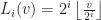


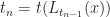


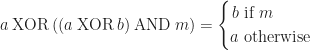
 algorithm in the obvious way. While it is not efficient for large problem sizes, it performs pretty well up to few hundred points.
 boxes was generated, and then sent to each library to compute a checksum of the set of pairs of intersections. Because different libraries expect their inputs in different formats, as a preprocessing step the boxes are converted into whatever data type is expected by the library. This conversion step is not counted towards the total running time. Note that the preparation phase does not include any time required to build associated data structures like search trees or grids; these timings are counted toward the total run time.
 , in order to avoid measuring the reporting time for each method.
 while constraining the boxes to remain within the unit hypercube,
 ![[0,1]^d](https://s0.wp.com/latex.php?latex=%5B0%2C1%5D%5Ed&bg=ffffff&fg=1a1a1a&s=0&c=20201002) . A typical sample from this distribution looks like this,
. A typical sample from this distribution looks like this,


 , but due to the constants involved is still far too slow. As it took too long and there were 2 other representatives of the r-tree data structure in the benchmark, I decided to drop it from larger tests. Moving on to 10k boxes,
 growth, however because the constants involved are so large they were also dropped from the large problem size.
 time of box-intersect. An explanation for this phenomenon would be that box-intersect enjoys better cache locality (scaling linearly with block size), while hashing causes
  indirect main memory accesses for each box. If the size of a cache line is
  , then the cross over point should occur when
  in 2D. This is illustrated in the following chart which carries out the experiment to 250k boxes,
 grid at each level of the tree along the quantiles. In the case of a uniform distribution of boxes, this reduces to uniform grid giving a query time of
 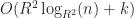 , which for finite
  gives means that rbush will find all intersections in
 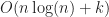 time. As a result, we can expect that once
  , rbush-bulk should eventually surpass box-intersect in performance (though this did not occur in my benchmarks). This also suggests another way to interpret the OMT heuristic: it is basically a hedged version of the uniform grid. While not quite as fast in the uniform case, it is more adaptive to sparse data.


 penalty, while adding robustness against sparse data.
 performance, as predicted.
 -axis by a factor of

 or
or  , then it would have been possible to increase their running times to some arbitrarily large value. In this benchmark, rbush also grows though by a much slower
  . Continuing out to 100k boxes, eventually rbush also fails,

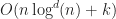 performance no matter what type of input you throw at it. It is even faster than grids for uniform distributions at small problem sizes(<10k) due to superior cache performance.
![[x_{min}, x_{max}] \times [y_{min}, y_{max}]](https://s0.wp.com/latex.php?latex=%5Bx_%7Bmin%7D%2C+x_%7Bmax%7D%5D+%5Ctimes+%5By_%7Bmin%7D%2C+y_%7Bmax%7D%5D&bg=ffffff&fg=1a1a1a&s=0&c=20201002) ).
).
![[x_0-r_0, x_0+r_0], [x_1-r_1, x_1+r_1]](https://s0.wp.com/latex.php?latex=%5Bx_0-r_0%2C+x_0%2Br_0%5D%2C+%5Bx_1-r_1%2C+x_1%2Br_1%5D&bg=ffffff&fg=1a1a1a&s=0&c=20201002) ,
,![[x_0-r_0, x_0+r_0] \cap [x_1-r_1, x_1+r_1] \neq \emptyset \Longleftrightarrow |x_0 - x_1| \leq r_0 + r_1](https://s0.wp.com/latex.php?latex=%5Bx_0-r_0%2C+x_0%2Br_0%5D+%5Ccap+%5Bx_1-r_1%2C+x_1%2Br_1%5D+%5Cneq+%5Cemptyset+%5CLongleftrightarrow+%7Cx_0+-+x_1%7C+%5Cleq+r_0+%2B+r_1&bg=ffffff&fg=1a1a1a&s=0&c=20201002)
![[l_0, h_0], [l_1, h_1]](https://s0.wp.com/latex.php?latex=%5Bl_0%2C+h_0%5D%2C+%5Bl_1%2C+h_1%5D&bg=ffffff&fg=1a1a1a&s=0&c=20201002) ,
,![[l_0, h_0] \cap [l_1, h_1] \neq \emptyset \Longleftrightarrow l_0 \leq h_1 \wedge l_1 \leq h_0](https://s0.wp.com/latex.php?latex=%5Bl_0%2C+h_0%5D+%5Ccap+%5Bl_1%2C+h_1%5D+%5Cneq+%5Cemptyset+%5CLongleftrightarrow+l_0+%5Cleq+h_1+%5Cwedge+l_1+%5Cleq+h_0&bg=ffffff&fg=1a1a1a&s=0&c=20201002)

 , then the amortized cost of looping over the events is
  . Therefore, the total running time of this algorithm is in
 .
. , then insert each of the boxes into the cells they overlap. Boxes which share a common grid cell are tested for overlaps:
 cells and that each cell contains at most
  (using a grid or hash table), or
 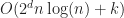 for sorted lists, which for small
  is effectively an optimal
 time, where
  .
.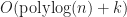 time, then it uses at least
 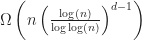 bits.
bits.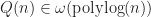 time per query. Therefore, the worst case time complexity of bvhIntersect is slower than,
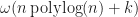 .
. time using
  and gave a construction which effectively matches this bound,
 , and for 3D
  .
. . Situations where the complexity degenerates to
  tend to be rare, and in practice applications can be designed to avoid them. Moreover, because R-trees have small space overhead and support fast updates, they are relatively cheap to maintain as an index. This has lead to them being used in many GIS applications, where the problem sizes make conserving memory the highest priority.
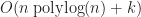 barrier in the worst case (with the exception of 1D interval sweeping and a brief digression into Shamos & Hoey’s algorithm). To the best of my knowledge, all efficient approaches to this problem make some essential use of
 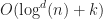 time using
 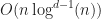 space (these results can be improved somewhat using
 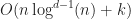 time.
time. . This approach is described in the following paper by Zomorodian and Edelsbrunner,
 is a n-by-d matrix
 is a m-by-d matrix
 is equivalent to the
  linear inequalities in

 time, which for fixed dimension is just
  . The dependence on
  using a more sophisticated data structure,
 . If this volume is
  , then the shapes collide. One way to compute this volume is to rewrite it as an integral. Let
  denote the
 in some basis, (for example, as Fourier waves), then we can use that to approximate this volume. If we do this expansion carefully, then with enough work we can show that the resulting approximation preserves something of the original geometry. For more details, here is a paper I wrote:
 (for comparison based algorithms) by reduction to the
  time using a
  , this is a big improvement over naive brute force. This technique can also be adapted to compute intersections in sets of general convex polygons by decomposing them into segments, and then building a secondary point location data structure to handle the case where a polygon is completely contained in another.
 called a
  = frequency of updates
 = the size of the game state
 bits/(second * player) or
  total bits. Clients have a downstream bandwidth of
  . Assuming a shared environment where every player sees the same state, then
  . This leaves us with two independent parameters,
  . Increasing
  .
. possible US phone numbers, and so any such number can be encoded in
  bits, or a little under 4 bytes. In general, given more type information it is possible to achieve smaller encodings.
 .
.  be the dimension of space and let
  denote a
  dimensional real vector space. In the
  into a spatial component
  and a
and a  . Now l
 be the maximum velocity any object can travel (aka the


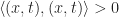
 . In this convention, causal vectors


 is a
is a 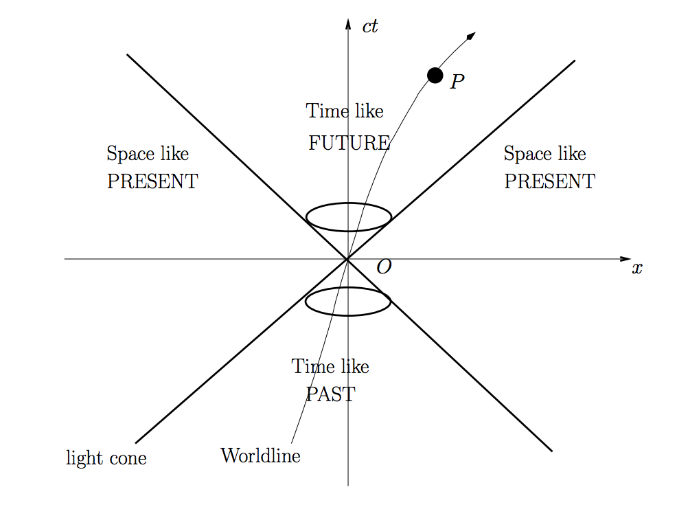
 we say that
  causally precedes
  (written
  ) if
) if  is future-directed causal or zero.
 is space-time consistent if for all
  ,
,  .
. determines a pair of closed regular sets called its causal future and causal past, respectively:

 . Conversely, events in
  .
.  is the light cone of
  ,
, .
. ,
, .
. which is the point in space-time at which it most recently received an input from its remote controller. Let
  be the set of all these events. We call the causal future
  the
the  . Consequently, these events can be predicted by dead-reckoning. On the other hand, events inside
 -dimensional collection of world lines in space-time into a

 ,
, .
. .
. determines a Cauchy surface is answered by the following theorem:
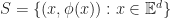 if and only if the subgradient of
  is bounded by
  .
. intersects the surface only once. To show that the curve crosses at least once, recall proposition 1 implies that
  and
and  , and that the curve begins in the causal past of
  be a point of intersection between the curve and the surface. Then the entire future of the curve is contained in the open cone
 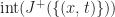 . Similarly, because
 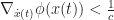 , no other points on
 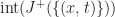 . Ditto for all the points in the causal past, and so any intersection must be unique. To show necessity, take any Cauchy surface
  as shown above. Suppose that there is some point
  and unit vector
  where
where  . Without loss of generality, assume
  . Then there exists some
  where
where 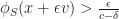 . Construct the time-like curve
 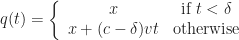 . By the intermediate value theorem,
  be the time of the oldest-most recent input from a remote player. Then define a constant Cauchy surface,
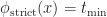 .
.
 be the time that the most recent local input was processed. Then the optimistic Cauchy surface is,
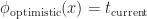 .
.

 , is the time that an event is rendered for a local user.
 varying as function of local time. We want to compute the time dilation experienced by an object with a coordinate time parameterized world line,
  . In this situation, define the mapping
  , that relates local time to the particle’s coordinate time,
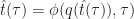 .
.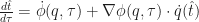 .
. , then objects will stop or possibly move backwards in time. This condition produces jitter, and it is important that we avoid it in all circumstances. Fortunately, it is not hard to derive a set of sufficient conditions to ensure that this is the case for all time-like paths:
 and
and  , then for any time-like particle the time dilation is strictly positive.
 , then for all
  ,
,  .
. , then for all
  ,
, 
 where
where 
 where,
 .
. the horizon. If the last locally processed input was at
  , then the minimum input delay of the local perception filter is,
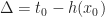 .
. is a function of the last acknowledged position and ping of all remote players. If
  , then we can respond to local inputs immediately. This leads to the following theorem which gives necessary conditions for a local input to be processed immediately:
 and their last acknowledged position is
  , then in order for a local perception filter to process a local input without lag, we must require that:
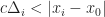

 distance from each other, then local perception filters completely eliminate input lag.
 .
.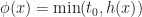
 is the time of the local player. Some other options would be to use a smoother surface or some offset of the true horizon. At any rate, this surface seems to give acceptable results but I fully expect that it could be improved drastically with more careful consideration.


 be the edges of a connected graph on
  we assign a weight
  which is the latency of the edge in seconds. In the network we assume that players only communicate with those whom are adjacent in
 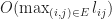 . The bandwidth required by active replication over a peer-to-peer network is
  per client, since each client must broadcast to every other client, or
  total.
 . The total bandwidth consumed is
  per client and
  for the server.
 , then we could conclude that peer-to-peer replication is overall more efficient. However, in practice this is not quite true for several reasons. First, in passive replication it is not necessary to replicate the entire state each tick, which results in a lower total bandwidth cost. And second, it is possible for clients to eagerly process inputs locally thus lowering the perceived latency. When applied correctly, these optimizations combined with the fact that it is easier to secure a client-server network against cheating means that it is in practice a preferred option to peer-to-peer networking.


