Peer-to-Peer Ordered Search Indexes

“Can we do to web services what Linux did to the operating systems?”

Imagine what the web with a P2P GitHub, a P2P YouTube, a P2P Twitter, a P2P Google search, and so on. But getting started with P2P services remains difficult, because:

“There is no P2P PostGRES!”

This is a very hard problem, so instead consider a more modest project:

“Let’s build a dynamic P2P ordered search index”

While pretty far from a full SQL database, a search index is a critical component for a modern RDBMS as it enables the following sorts of queries:

  • Predecessor/successor
  • Range search
  • ORDER-BY
  • Multi column joins
  • …and much more

In this post we’ll talk about a few standard solutions to this problem, explain why they don’t work so well in P2P systems and finally we’ll present an idea that both simplifies these data structures and solves these problems.

Quick review: Merkle DAGs

For the uninitiated, building robust P2P systems seems like an impossible problem. How do you build anything if you can’t trust your peers? Well, cryptographers have known how to do this more than 60 years using a technique I’ll call Merkleization.

R. Merkle (1979) “A Certified digital signature

Merkleization turns certain kinds of data structures into “invincible” P2P versions, and can be described in just 4 words:

Replace pointers with hashes

Merkleization is the active ingredient in BitTorrent, Git, IPFS and BitCoin‘s block chain. Using hashes we can validate any sequence of reads from a common data structure as long as we trust the root hash.  This allows us to use any form of content addressable storage like a DHT or some other P2P network fetch arbitrary data, with no need to trust the network or storage layers. Such data structures can also work offline if the necessary data is cached locally. The worst case failure is that the data structure simply becomes temporarily unavailable if we can’t find a hash.

Because the objects in a Merkleized data structure are referenced using hashes, they are effectively immutable. These references must be created in causal order, and so they form a directed acyclc graph, hence the term Merkle DAG. All Merkle DAGs are functional data structures, and any functional data structure can be turned into a Merkle DAG by Merkleization. Updates to Merkle-DAGs can be performed using path-copying techniques as described in Okasaki’s PhD thesis:

C. Okasaki (1996) “Purely functional data structures” PhD Thesis

Merkle DAGs are an example of an authenticated data structure, which means that they support queries answered by untrusted 3rd parties. The trusted writer to the data structure only needs to provide the root hash to certify the correctness of sequences of queries from the reader. A more recent treatment of Merkle DAGs from the perspective of programming languages can be found here:

A. Miller, M. Hicks, J. Katz, E. Shi. (2014) “Authenticated data structures, generically” POPL

Merkle DAGs are pretty great, but they do have some limitations. The following general problems are universal to all functional data structures:

  • Nodes are created in causal order, so no cycles are possible (ie no doubly linked lists)
  • Changes by path copying are more expensive than in mutable data structures
  • Objects are finite size. No O(1) RAM arrays (and no bucket sort, and so on)
  • We have to deal with garbage collection somehow or else let objects slowly fill up storage… (Reference counting and freeing nodes induces side effects)

Still, they also get some cool benefits:

  • Merkle DAGs are functionally persistent, we can easily rollback to old versions, fork them and even merge them efficiently
  • Checking the equality of two Merkle DAGs is an O(1) operation — just compare their hashes!
  • They’re authenticated (works with P2P)
  • They’re simple!

B-trees

Now let’s return to ordered search indexes. A typical RDBMS would use some variation of a B-tree, and since B-trees don’t contain cycles we can Merkelize them, which has of course been done:

Y. Yang, D. Papadias, S. Papadopolous, P. Kalnis. (2009) “Authenticated Join Processing in Outsourced Databases” SIGMOD

However, it turns out that while B-trees are great in an imperative environment run on a trusted host, they are not ideal as a P2P functional data structure. One problem is B-tree implementations typically rely on amortized vacuuming/rebalancing in order to keep queries fast after many deletes, which can be expensive in a P2P setting. A second related issue is that the structure of a B-tree depends significantly on the order of insertion. Some databases implement mechanisms like “BULK INSERT” for sequentially inserting elements into a B-tree to avoid the performance degradation caused by many half-filled nodes.

Fundamentally, these problems are all aspects of a phenomenon I shall call hysteresis by analogy to systems theory:

Defn: A data structure for maintaining a dynamic ordered set of elements under insertion and removal has hysteresis if the history of updates determines the state of the data structure irrespective of the underlying set.

Data structures with hysteresis have path dependency, in the case of B-trees the actual tree structure depends on the order of inserts and removes. This means that B-trees are non-canonical, there is more than one way to encode any given sequence in a B-tree (ie there is extra information stored in the structure of the tree). This significantly limits what can be done to process indexes offline; for a B-tree you must reprocess all updates on the tree in the exact order of the writer to verify its computations. Finally, we can’t take full advantage of structure sharing to deduplicate common subsequences in trees or test the quality of two B-trees by comparing hashes. Of course, B-trees are not exceptional in this regard. Many other common search trees suffer from similar problems, including Red-Black trees, AVL-trees, Splay trees and so on.

Merkle Search trees

Fortunately, we can solve all the above problems at once if we can find some way to make the tree structure deterministic: that is any reordering of the same elements should produce the same data structure. It seems that deterministic authenticated search trees were first studied by Auvolat and Taïani:

A. Auvolat, F. Taïani. (2019) “Merkle Search Trees: Efficient State-Based CRDTs in Open Networks

Merkle Search Trees are an incremental method for constructing determinstic B-trees. Their idea is to first hash all content which is inserted into the tree, and then to place items at a level proportional to the number of 0’s in the prefix of their hash written in base B. Under the assumption that all hashes are uniformly distributed, a Merkle search tree has the following properties:

  1. Every internal node has on average B children
  2. All leaves are on average the same distance from the root
  3. The tree is deterministic

Bottom up Chunking

Merkle search trees have some nice properties, but insertions and removal from them can be complex. Updates to a Merkle search tree proceed by traversing the tree top-to-bottom and locating an item based on its key and hash values. Instead we propose directly constructing trees from the bottom up, building up the tree layer-by-layer as chunked sorted lists of hashes. The data we are considering will always be arrays of k-bit hashes; either lists of pointers to nodes, or pointers to hashes of values, and so we can make a cut after any hash whose binary value is less than 2^k / B:

function nextChunk (hashes, start) {
  for (let i = start; i < hashes.length; ++i) {
    if (hashes[i] < pow(2, HASH_BITS) / B) {
      return i;
    }
  }
  return hashes.length;
}

This chunking procedure is similar to the content-defined chunking method used by the rsync backup system developed Tridgell in his PhD Thesis:

> A. Tridgell, (1999) “Efficient Algorithm for Sorting and Synchronization” PhD Thesis

Uniform distribution of hashes implies that the block sizes will follow a mean-B Poisson distribution and so almost all blocks are \Theta(B). These cuts are robust under insertions and deletions of nodes, since each cut depends only on the value of its own hash. Putting it all together, we get the following psuedo-code:

// assume items is a sorted array of (key, value) pairs
function createBTree (items) {
  let hashes = items.map(storeLeaf);
  do {
    let nextHashes = []
    for (let lo = 0; lo < hashes.length; ) {
       // use the previous method to find the next chunk
       let hi = nextChunk(hashes, lo);
       nextHashes.push(storeNode(hashes.slice(lo, hi)));
       lo = hi;
    }
    hashes = nextHashes;
  } while (hashes.length !== 1)
  return hashes[0];
}

Under the above assumptions, this should give a tree which is height at most O(\log_B(n)), and so createBTree terminates after O(\log_B(n)) for a total cost of O(n \log_B(n)) time and O(\frac{n}{B} \log_B(n)) nodes. Authenticated queries against this tree are again O(log_B(n)) and can use the standard B-tree search procedure.

Even better, updates to these trees aren’t too expensive: In general, for any update/insert/delete operation, we first locate the block containing the elements we are modifying, then we rewrite those blocks as well as any nodes along its root-to-leaf path. Because of our chunking criteria, the extent of this modification changes no other nodes besides those along the root-to-leaf path, and so expected cost is O(\frac{m}{B} \log_B(n + m), where m is the total number of elements modified.

Conclusion

Merkle search trees are a promising direction for future investigations into peer-to-peer database indexes. Content chunking is generally applicable to many other types of search tree data structures, including for example R-trees and suffix arrays.

However, there remain some unsolved issues with both this approach and Merkle Search trees.  A big problem is that neither are secure against adversarial inputs. A malicious writer could easily overflow a block with selected hashes, or inflate the tree height by brute forcing a prefix (though our bottom up construction is more resistant to this latter attack).  Still this is a promising direction for peer-to-peer search indexes and suggests that scalable, fully authenticated functional databases may be possible in the future.

Acknowledgements

This project was supported by Protocol Labs LLC and jointly created with the help of Mikeal Rogers, who is the lead of the IPLD project at Protocol Labs.
Texture atlases, wrapping and mip mapping

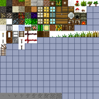
Today I want to write about what is probably the single most common question that gets asked regarding greedy meshes.  Specifically: How can greedy meshes be texture mapped? One naive solution might be to create a separate texture for each block type, and then do a separate pass for each of these textures.  However, this … Continue reading “Texture atlases, wrapping and mip mapping”

Today I want to write about what is probably the single most common question that gets asked regarding greedy meshes.  Specifically:

How can greedy meshes be texture mapped?

One naive solution might be to create a separate texture for each block type, and then do a separate pass for each of these textures.  However, this would require a number of state changes proportional to O(number of chunks * number of textures).  In a world with hundreds of textures and thousands of chunks, this would be utterly unacceptable from a performance standpoint.  Instead, a better solution is to use a technique called texture atlases.

Texture Atlases

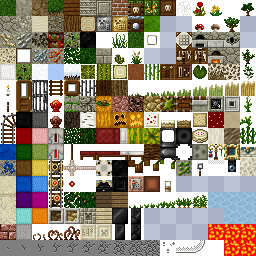
Now if you’ve ever modded Minecraft or looked inside a texture pack from before 1.5, the concept of a texture atlas should be pretty straightforward.  Instead of creating many different textures, an atlas packs all of the different textures into a single gigantic texture:

An example of a texture atlas for Minecraft.  (c) 2009 rhodox.
An example of a texture atlas for Minecraft. (c) 2013 rhodox.

Texture atlases can greatly reduce the number of draw calls and state changes, especially in a game like Minecraft, and so they are an obvious and necessary optimization. Where this becomes tricky is that in order to get texture atlases to work with greedy meshing, it is necessary to support wrapping within each subtexture of the texture atlas.  In OpenGL, there are basically two ways to do this:

  1. Easy way: If your target platform supports array textures or some similar extension, then just use those, set the appropriate flags for wrapping and you are good to go!
  2. Hard way: If this isn’t an option, then you have to do wrapping and filtering manually.

Obviously the easy way is preferable if it is available.  Unfortunately, this isn’t the case for many important platforms like WebGL or iOS, and so if you are writing for one of those platforms then you may have to resort to an unfortunately more complicated solution (which is the subject of this blog post).

Texture Coordinates

The first problem to solve is how to get the texture coordinates in the atlas.  Assuming that all the voxel vertices are axis aligned and clamped to integer coordinates, this can be solved using just the position and normal of each quad.  To get wrapping we can apply the fract() function to each of the coordinates:

vec2 tileUV = vec2(dot(normal.zxy, position), 
                   dot(normal.yzx, position))
vec2 texCoord = tileOffset + tileSize * fract(tileUV)

Here the normal and position attributes represent the face normal and position of each vertex.  tileOffset is the offset of the block’s texture in the atlas and tileSize is the size of a single texture in the atlas.  For simplicity I am assuming that all tiles are square for the moment (which is the case in Minecraft anyway).  Taking the fract() causes the texture coordinates (called texCoord here) to loop around.

Mipmapping Texture Atlases

Now the above technique works fine if the textures are filtered using GL_NEAREST or point filtering.  However, this method quickly runs into problems when combined with mipmapping.  There are basically two things that go wrong:

  1. Using an automatic mipmap generator like glGenerateMipmaps will cause blurring across texture atlas boundaries, creating visible texture seams at a distance.
  2. At the edge of a looped texture the LOD calculation will be off, and causing the GPU to use a much lower resolution mip level than it should.

At least the first of these problems is pretty easy to solve.  The simple fix is that instead of generating a mipmap for all the tiles simultaneously, we generate a mipmap for each tile independently using periodic boundary conditions and pack the result into a texture map.  This can be done efficiently using sinc interpolation and an FFT (for an example of how this works, check out this repository).  Applying this to each tile in the texture atlas separately prevents any accidental smearing across boundaries.  To compare, here are side-by-side pictures of standard full texture mipmapping compared to correct per-tile periodic mipmaps:

0Base Tilesheet

Left: Per-tile mipmap with wrapping.     Right: Naive full texture mipmap.

Mipmap Level 1         Mipmap without tile

Level 1

Mip2tile         Mip2NoTile

Level 2

Mip3Tile        Mip3NoTile

Level 3

Mip4Tile      Mip4NoTile

Level 4

If you click and zoom in on those mipmaps, it is pretty easy to see that the ones on the left side have fewer ringing artefacts and suffer bleeding across tiles, while the images on the right are smeared out a bit.  Storing the higher mip levels is not strictly necessary, and in vanilla OpenGL we could use the GL_TEXTURE_MAX_LEVEL flag to avoid wasting this extra memory.  Unfortunately on WebGL/OpenGL ES this option isn’t available and so a storing a mipmap for a texture atlas can cost up to twice as much memory as would be required otherwise.

The 4-Tap Trick

Getting LOD selection right requires a bit more creativity, but it is by no means insurmountable.  To fix this problem, it is first necessary to understand how texture LODs are actually calculated.  On a modern GPU, this is typically done by looking at the texture reads within a tiny region of pixels on the screen and then selecting a mip level based on the variance of these pixels.  If the pixels all have very large variance, then it uses a higher level on the mip pyramid, while if they are close together it uses a lower level.  In the case of our texture calculation, for most pixels this works well, however at the boundary of a tile things go catastrophically wrong when we take the fract():

Texture tiling seams caused by incorrect LOD selection.  Note the grey bars between each texture.
Texture tiling seams caused by incorrect LOD selection. Note the grey bars between each texture.

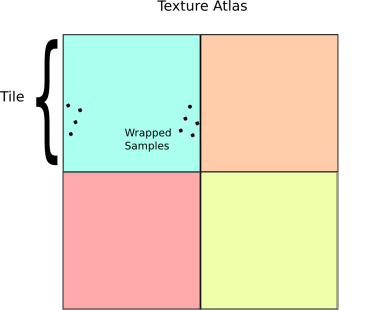
Notice the grey bars between textures.  In actual demo the precise shape of these structures is view dependent and flickers in a most irritating and disturbing manner.  The underlying cause of this phenomenon is incorrect level of detail selection.  Essentially what is happening is that the shader is reading texels in the following pattern near the edges:

Texture access near a tile boundary.  Note how the samples are wrapped.
Texture access near a tile boundary. Note how the samples are wrapped.

The GPU basically sees this access pattern, and think: “Gosh!  Those texels are pretty far apart, so I better use the top most mip level.”  The result is that you will get the average color for the entire tile instead of a sample at the appropriate mip level.  (Which is why the bands look grey in this case).

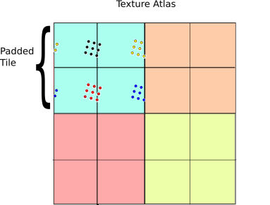
To get around this issue, we have to be a bit smarter about how we access our textures.  A fairly direct way to do this is to pad the texture with an extra copy of itself along each axis, then sample the texture four times:

The 4-tap algorithm illustrated.  Instead of sampling a single periodic texture once, we sample it 4 times and take a weighted combination of the result.
The 4-tap algorithm illustrated. Instead of sampling a single periodic texture once, we sample it 4 times and take a weighted combination of the result.

The basic idea behind this technique is a generalized form of the pigeon hole principle.  If the size of the sample block is less than the size of  the tile, then at least one of the four sample regions is completely contained inside the 2×2 tile grid.  On the other hand, if the samples are spread apart so far that they wrap around in any configuration, then they must be larger than a tile and so selecting the highest mip level is the right thing to do anyway.  As a result, there is always one set of samples that is drawn from the correct mip level.

Given that at least one of the four samples will be correct, the next question is how to select that sample?  One simple solution is to just take a weighted average over the four samples based on the chessboard distance to the center of the tile.  Here is how this idea works in psuedo GLSL:

vec4 fourTapSample(vec2 tileOffset, //Tile offset in the atlas 
                  vec2 tileUV, //Tile coordinate (as above)
                  float tileSize, //Size of a tile in atlas
                  sampler2D atlas) {
  //Initialize accumulators
  vec4 color = vec4(0.0, 0.0, 0.0, 0.0);
  float totalWeight = 0.0;

  for(int dx=0; dx<2; ++dx)
  for(int dy=0; dy<2; ++dy) {
    //Compute coordinate in 2x2 tile patch
    vec2 tileCoord = 2.0 * fract(0.5 * (tileUV + vec2(dx,dy));

    //Weight sample based on distance to center
    float w = pow(1.0 - max(abs(tileCoord.x-1.0), abs(tileCoord.y-1.0)), 16.0);

    //Compute atlas coord
    vec2 atlasUV = tileOffset + tileSize * tileCoord;

    //Sample and accumulate
    color += w * texture2D(atlas, atlasUV);
    totalWeight += w;
  }

  //Return weighted color
  return color / totalWeight
}

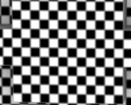
And here are the results:

No more seams!  Yay!
No more seams! Yay!

Demo

All this stuff sounds great on paper, but to really appreciate the benefits of mipmapping, you need to see it in action.  To do this, I made the following demo:

http://mikolalysenko.github.io/voxel-mipmap-demo/

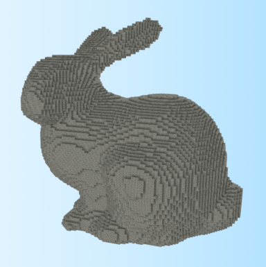
And here is a screenshot:

Voxel mipmap demoSome things to try out in the demo are displaying the wireframes and changing the mip map filtering mode when zooming and zooming out.  The controls for the demo are:

  • Left click: Rotate
  • Right click/shift click: Pan
  • Middle click/scroll/alt click: Zoom

The code was written using browserify/beefy and all of the modules for this project are available on npm/github.  You can also try modifying a simpler version of the above demo in your browser using requirebin:

http://requirebin.com/?gist=5958022

Conclusion

In conclusion, greedy meshing is a viable strategy for rendering Minecraft like worlds, even with texture mapping.  One way to think about greedy meshing from this perspective is that it is a trade off between memory and vertex shader and fragment shader memory. Greedy meshing drastically reduces the number of vertices in a mesh that need to be processed by merging faces, but requires the extra complexity of the 4-tap trick to render.  This results in lower vertex counts and vertex shader work, while doing 4x more texture reads and storing 4x more texture memory. As a result, the main performance benefits are most important when rendering very large terrains (where vertex memory is the main bottleneck).  Of course all of this is moot if you are using a system that supports texture arrays anyway, since those completely remove all of the additional fragment shader costs associated with greedy meshing.

Another slight catch to the 4-tap algorithm is that it can be difficult to implement on top of an existing rendering engine (like three.js for example) since it requires modifying some fairly low level details regarding mipmap generation and texture access.  In general, unless your rendering engine is designed with some awareness of texture atlases it will be difficult to take advantage of geometry reducing optimizations like greedy meshing and it may be necessary to use extra state changes or generate more polygons to render the same scene (resulting in lower performance).

CommonJS: Why and How

As I said last time, I want to start moving more of my stuff into npm, and so I think perhaps today would be a good time to explain why I think this is the right way to go, and how you can use it in your own JS projects.

The big picture reason that all of this stuff is important, is that there a huge trend these days towards single page browser based applications and JavaScript development in general.  Many factors have contributed to this situation, like the rise of fast JavaScript interpreters; widespread frustration and distrust of web plugins like SilverlightJava Applets and Flash; and the emergence of powerful new APIs like HTML 5 and WebGL.  Today, JavaScript runs on pretty much everything including desktops, cell phones, tablets and even game consoles.  Ignoring it is something you do at your own risk.

Module Systems

However, while there are many good reasons to use JavaScript, it has a reputation for scaling poorly with project size.  In my opinion, the main cause of this is that JavaScript lacks anything even remotely resembling a coherent module system.  This omission makes it inordinately difficult to apply sensible practices like:

  • Hiding implementation details behind interfaces
  • Splitting large projects into multiple files
  • Reusing functionality from libraries and other code bases

Ignoring these problems isn’t an option.  But despite its flaws, JavaScript deserves at least some credit for being a very flexible language, and with some ingenuity one can work around the lack of modules.  There are of course many ways you can do this, and for me at least as I’ve been learning JS I’ve found the bewildering array of solutions pretty confusing.  So in this post I’m going to summarize how I understand the situation right now, and give my assessment of the various options:

Ad-Hoc

The obvious way to emulate a module in JavaScript would be to use a closure.  There is a fancy name for this in the JS community, and it is called the module design pattern:

var MyModule = (function() {
  var exports = {};
  //Export foo to the outside world
  exports.foo = function() {
   // ...
  }

  //Keep bar private
  var bar = { /* ... */ };

  //Expose interface to outside world
  return exports;
})();

Here MyModule would become the interface for the module and the implementation of the module would be hidden away within the function() block.  This approach, when combined with features like “use strict”; can go a long way to mitigating the danger of the global-namespace free-for-all; and if applied with discipline it basically solves the first problem on our big list.

Unfortunately, it doesn’t really do much to fix our multiple files or importing problems.  Without bringing in third party tools or more complex module loaders, you are basically limited to two ways to do this within a browser:

  • You can add each of your JS files using a <script> in your header.
  • Or you can just concatenate all your files in a static build process.

The latter approach is generally more efficient since it requires fewer HTTP requests to load and there are tools like Google’s closure compiler which support this process.  The former approach is more dynamic since you can develop and test without having to do a full rebuild.  Unfortunately, neither method lets you to do selective imports, and they don’t handle external dependencies across libraries very well.

This style of coding is sometimes called monolithic, since the pressure to avoid code dependencies tends to push projects written in this fashion towards monumental proportions.  As an example, look at popular libraries like jQuery, YUI or THREE.js, each of which is packed with loads of features.  Now I don’t mean to especially pick on any of these projects, since if you aren’t going to accept external tooling their approach is actually quite reasonable.  Packaging extra functionality into a library (in the absence of a proper importing system) means you get a lot more features per <script>.  Sufficiently popular libraries (like jQuery) can leverage this using their own content distribution networks and can be cached across multiple sits.  This is great for load times, since users then don’t have to re-download all those libraries that their browser already has cached when they go from site-to-site.

The cost though is pretty obvious.  Because <script> tags have no mechanism to handle dependencies, the default way to include some other library in your project is copy-paste.  Heavy use of this style is a great way to proliferate bugs, since if you include a library with your project via this mechanism, you usually have no good way to automatically update it.

CommonJS

The CommonJS module system solves all these problems.   The way it works is that instead of running your JavaScript code from a global scope, CommonJS starts out each of your JavaScript files in their own unique module context (just like wrapping it in a closure).  In this scope, it adds two new variables which you can use to import and export other modules: module.exports and require.  The first of these can be used to expose variables to other libraries.  For example, here is how to create a library that exports the variable “foo”:

//In library.js
exports.foo = function() {
    //... do stuff
}

And you can import it in another module using the “require” function:

var lib = require("./library.js");
lib.foo();

The addition of this functionality effectively solves the module problem in JavaScript, in what I would consider the most minimally invasive way.  Today, CommonJS is probably the most widely adopted module system in JavaScript, in part due to the support from node.js.  The other major factor which has contributed to its success is the centralized npm package manager, which makes it easy to download, install and configure libraries written using CommonJS.

CommonJS packages should be lean and mean, with as little extraneous functionality as possible.  Compare for example popular modules like async or request to monolithic libraries like underscore.js or jQuery.  An interesting discussion of this philosophy can be found at James Halliday (substack)’s blog:

J. Halliday, “the node.js aesthetic” (2012)

Based on the success of node.js, this approach seems to be paying off for writing server side applications.  But what about browsers?

CommonJS in the Browser

It turns out that doing this directly isn’t too hard if you are willing to bring in an extra build process.  The most tool to do this is browserify.  When you run browserify, it crawls all your source code starting from some fixed entry point and packages it up into a single .js file, which you can then minify afterwords (for example, using uglify.js).  Doing this reduces the number of http requests required to start up a page and reduces the overall size of your code, thus improving page load times.  The way it works is pretty automatic, just take your main script file and do:

browserify index.js > bundle.js

And then in your web page, you just add a single <script> tag:

<script src="bundle.js"></script>

browserify is compatible with npm and implements most of the node.js standard library (with the exception of some obviously impossible operating system specific stuff, like process.spawn).

Rapid Development with browserify

The above solution is pretty good when you are looking to package up and distribute your program, but what if you just want to code and debug stuff yourself with minimal hassle? You can automate the bulk of this process using a Makefile, but one could argue reasonably that having to re-run make every time you edit something is an unnecessary distraction.  Fortunately, this is a trivial thing to automate, and so I threw together a tiny ~100-line script that runs browserify in a loop.  You can get it here:

serverify – Continuous development with browserify

To use it, you can just run the file from your project’s root directory and it will server up static HTML on port 8080 from ./www and bundle up your project starting at ./index.js. This behavior can of course be changed by command line options or configuration files.  As a result, you get both the advantages of a proper module system and the ease of continuous deployment for when you are testing stuff!

Other Formats

As it stands today, CommonJS/npm (especially when combined with tools like browserify) is an efficient and  comprehensive solution to the module problem in JavaScript.  In my opinion, it is definitely the best option if you are starting out from scratch.  But I’d be remiss if I didn’t at least mention some of the other stuff that’s out there, and how the situation may change over time:

  • Looking ahead to the distant future, ECMA Script 6 has a proposal for some new module semantics that seems promising.  Unfortunately, we aren’t there yet, and no one really knows exactly what the final spec will look and how far out it will be until it gets there.  However, I hope that someday they will finally standardize all of this stuff and converge on a sane, language-level solution to the module problem.  For a balanced discussion of the relative merits of the current proposal,  I’d recommend reading the following post by Isaac Schlueter (current maintainer of node.js):

Schlueter, I. “On ES6 Modules” (2012)

    1. Special syntax for specifying module imports (must be done at the top of each script)
    2. No tooling required to use, works within browsers out of the box.

These choices are motivated by a preceived need to get modules to work within browsers with no additional tooling.  The standard reference implementation of AMD is the RequireJS library, and you can install it on your sever easily by just copy/pasting the script into your wwwroot.

The fact that AMD uses no tools is both its greatest strength and weakness.  On the one hand, you can use it in a browser right away without having to install anything. On the other hand, AMD is often much slower than CommonJS, since you have to do many async http requests to load all your scripts.  A pretty good critique of the AMD format can be found here:

Dale, T. “AMD is not the answer

I generally agree with his points, though I would also like to add that a bigger problem is that AMD does not have a robust package manager.  As a result, the code written for AMD is scattered across the web and relies on copy-paste code reuse.  There are some efforts under way to fix this, but they are nowhere near as advanced as npm.

Conclusion

I’ve now given you my summary of the state of modules in JavaScript as I understand it, and hopefully explained my rationale for why I am picking CommonJS for the immediate future.  If you disagree with something I’ve said, have any better references or know of something important that I’ve missed, please leave a comment!

New Year’s Resolution: Post more stuff on npm

First thing, I’d like to help announce/promote a project which I think is pretty cool (but am not directly involved in) which is voxeljs.  It is being developed by @maxogden and @substack, both of which are very active in the node.js community.  Internally, it uses some of the code from this blog, and it looks super fun to hack around with.  I highly recommend you check it out.

Second, I’d like to say that from here on out I’m going to try to put more of my code on npm so that it can be reused more easily.  I’m going to try to focus on making more frequent, smaller and focused libraries, starting with an npm version of my isosurface code:

https://github.com/mikolalysenko/isosurface

In the future, I hope to start moving more of my stuff on to npm, piece by piece.  Stay tuned for more details.

Changed WordPress Theme

I was getting a bit tired of the old theme I was using (Manifest) and decided to try something different.  One nice thing with this new version is that it has a sidebar which makes it a bit easier to navigate around the blog.  I’m also going to be adding some links to other blogs and resources on the sidebar over time.

If anyone has some further suggestions or ideas, please leave a comment!

Ludum Dare 21 Results

Well the results for Ludum Dare 21 are in!  Here is the final rank for my entry:

Ratings

#4 Innovation(Jam) 3.90
#29 Overall(Jam) 2.95
#30 Humor(Jam) 2.33
#31 Graphics(Jam) 3.30
#32 Fun(Jam) 2.55
#45 Audio(Jam) 2.12
#60 Coolness 8%
#63 Theme(Jam) 2.40
#104 Community 3.13

I have to say that I am a bit disappointed about only getting 4th place for innovation 😦 .  (At least I got in the top 10 in that category, which is somewhat respectable given the huge number of entries!)  I think that the controls definitely could have been done a bit better.  In retrospect it was a mistake to use a separate parallel transport frame for moving the camera and for applying forces.  This caused the camera to drift slightly which made the controls more confusing than they needed to be (plus it would have been a really easy fix had I thought of it during the competition).  I’m not sure if it is worth developing this concept into a full game.  Judging by the rating, it didn’t seem like it was that popular, but perhaps I am reading too much into the scores.  Also I think that the screen shot I picked for the entry was not nearly exciting enough (the wood level would have been much better), and the some of the levels definitely needed more polish.

At least there is a mini-LD coming up next weekend, so hopefully that will go a bit better!

New paper out!

Haven’t updated this blog in a long time, but I figure that since it is summer now maybe I will finally be able to keep this thing regularly updated (see how long that lasts…)  Anyway, some good news is that my latest paper has been accepted to the SIAM/SIGGRAPH conference on solid and physical modeling.  Here is a link to the download:

http://sal-cnc.me.wisc.edu/index.php?option=com_remository&Itemid=143&func=fileinfo&id=183

There’s a bunch of neat ideas in here, but the big idea here is the Minkowski product.  The motivation for this comes from the basic Minkowski sum.  If we recall, for two sets A, B \subseteq \mathbb R^n, their Minkowski sum is defined as:

A \oplus B = \{ a + b | a \in A, b \in B \}

Or alternatively,

A \oplus B = \bigcup \limits_{a \in A} a + B

The idea behind the Minkowski product is to replace \mathbb R^n with an arbitrary group, G.  If we do this, then we can define the Minkowski product over G in the following way:

A \stackrel{G}{\otimes} B = \bigcup \limits_{a \in A} a B

Much like how the Minkowski sum is useful for collision detection of translating objects, the generalized Minkowski product can be used for collision detection between translating and rotating bodies.  Similarly, we can also define a Minkowski quotient which is analogous to the Minkowski difference:

A \stackrel{G}{\oslash} B = \bigcap \limits_{a \in A} a B

And even better yet, we show how to compute these quantities using convolution algebras!  These operators turn out to be very useful in understanding things like partial symmetries of solids, mechanism workspaces and robotics.  All of the gory details and more are in the paper!

Hello World

Hi.  My name is Mikola Lysenko and this is my first post on 0FPS. I am currently a first year graduate student at the University of Wisconsin-Madison, working in the spatial automation lab.  I used to run the website assertfalse.com, but I ended up taking it down to save money on bandwidth expenses.  Anyway, I figure that lately I’ve been too lazy in my writing process and that a blog is a pretty good way to bring discipline back into my life.  I intend to focus on research topics in solid modeling and computer graphics, as well as other ideas I find interesting.