Shapes and Coordinates

In a previous post, I talked a bit about solid modeling and discussed at a fairly high level what a solid object is.  This time I’m going to talk in generalities about how one actually represent shapes in practice.  My goal here is to say what these things are, and to introduce a bit of physical language which I think can be helpful when talking about these structures and their representations.

The parallel that I want to draw is that we should think of shape representations in much the same way that we think about coordinates.  A choice of coordinate system does not change the underlying reality of the thing we are talking about, but it can reveal to us different aspects of the nature of whatever it is we are studying.  Being conscious of the biases inherent in any particular point of view allows one to be more flexible when trying to solve some problem.

Two Types of Coordinates

I believe that there are two general ways to represent shapes: Eulerian and LagrangianI’ll explain what this all means shortly, but as a brief preview here is a small table which contrasts these two approaches:

Eulerian Lagrangian
Coordinate System Global/fixed Local/moving
Modeling Paradigm Implicit Parametric
Transforms Passive Active

Eulerian (Implicit)

The first of these methods, or the Eulerian representation, seeks to describe shapes in terms of the space they embedded in.  That is shapes are described by maps from an ambient space into a classifying set:

f : \mathrm{Ambient}\:\mathrm{space} \to \mathrm{Classifying}\:\mathrm{space}

More concretely, suppose we are working in n-dimensional Euclidean space \mathbb{R}^n.  As we have already seen, it is possible to describe solids using sublevel sets of functions.  At a high level, the way this works is that we have some map f : \mathbb{R}^n \to S where S is some set of labels, for example the real line \mathbb{R}.  Then we can define our shape as the preimage of some subset of these labels, S_0 \subset S:

X = f^{-1}(S_0)

Again, if S = \mathbb{R} and S_0 = (-\infty, 0], then we get the usual definition of a sublevel set:

X = f^{-1}([-\infty, 0)) = \{ x \in \mathbb{R}^n : f(x) < 0 \} = V_0(f)

But these are of course somewhat arbitrary choices.  We could for example replace \mathbb{R} with the set S = \{ 0,1 \} of truth values, and we might consider defining our shape as the preimage of 1:

X = f^{-1}(1)

Which would be the set of all points in \mathbb{R}^n where f evaluates to 1.  In this situation f is what we could all point membership function.

Examples of Eulerian Representations

Motion in an Eulerian System

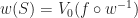
Say we have some Eulerian representation of our shape and we want to move it around.  One simple way to think about this is that we have the shape and we simply apply some map w : \mathbb{R}^n \to \mathbb{R}^n to warp it into a new position:

Moving a shape by a map

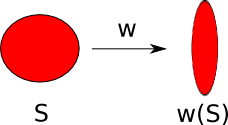
I probably don’t need to convince you too much that motions are extremely useful in animation and physics, but they can also be a practical way to model shapes.  In fact, one simple way to construct more complicated shapes from simpler ones is to deform them along some kind of motion.  Now here is an important question:

Question: How do we apply a motion in an Eulerian coordinate system?

Or more formally, suppose that we have a set S \subseteq \mathbb{R}^n and we have some warp w : \mathbb{R}^n \to \mathbb{R}^n.  If S = f^{-1}( [-\infty, 0) is the 0-sublevel set of some potential function f, can we find another potential function h such that,

h^{-1}( [ -\infty, 0 ) ) = w(S)

If you’ve never thought about this before, I encourage you to pause for a moment to think about it carefully.

Done?  Ok, here is how we can arrive at the answer by pure algebraic manipulation.  Starting with the definition for S, we get:

h^{-1}( . ) = w( f^{-1}( . ) )

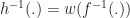
And taking inverses on both sides,

h( x ) = f( w^{-1}( x ) )

Which is of course only valid when w is invertible.  So in summary,

In an Eulerian coordinate system, to move a shape S = V_0(f) by w, we must precompose f with $w^{-1}$:

w(S) = V_0(f \circ w^{-1})

Or said another way:

Eulerian coordinate systems transform passively.

Pros and Cons

There are many advantages to an Eulerian coordinate system.  For example, point wise operations like Boolean set operations are particularly easy to compute.  (Just taking the min/max is sufficient to evaluate set intersection/union.)  On the other hand, because Eulerian coordinates are passive, operations like rendering or projection (which are secretly a kind of motion) can be much more expensive, since they require solving an inverse problem.  In general, this is as hard as root finding and so it is a non-trivial amount of work.  In 3D, there is also the bigger problem of storage, where representations like voxels can consume an enormous amount of memory.  However, in applications like image processing the advantages often outweigh the costs and so Eulerian representations are still widely used.

Lagrangian (Parametric)

Lagrangian coordinates are in many ways precisely the dual of Eulerian coordinates.  Instead of representing a shape as a map from an ambient space to some set of labels, they instead map a parametric space into the ambient space:

p : \mathrm{Parameter}\: \mathrm{space} \to \mathrm{Ambient}\: \mathrm{space}

The simplest example of a Lagrangian representation is a parametric curve, which typically acts by mapping an interval (like [0,1]) into some ambient space, say \mathbb{R}^n:

p(t) = ( x(t), y(t), z(t) )

But there are of course more sophisticated examples.  Probably the most common place where people bump into Lagrangian coordinates is in the representation of triangulated meshes.  A mesh is typically composed of two pieces of data:

  1. A cell complex (typically specified by the vertex-face incidence data)
  2. And an embedding fo the cell complex into \mathbb{R}^3

The embedding is commonly taken to be piecewise linear over each face.  There are of course many examples of Lagrangian representations:

Examples of Lagrangian Representations:

Motion in Lagrangian Coordinates

Unlike in an Eulerian coordinate system, it is relatively easy to move an object in a Lagrangian system, since we can just apply a motion directly.  To see why, let p : P \to \mathbb{R}^n be a parameterization of a shape S and let w : \mathbb{R}^n \to \mathbb{R}^n be a motion; then obviously:

w(S) = w(p(P)) = (w \circ p)(P)

And so we conclude,

Lagrangian coordinate systems transform actively.

Pros and Cons

The main advantage to a Lagrangian formulation is that it is much more compact than the equivalent Eulerian form when the shape we are representing is lower dimensional than the ambient space.  This is almost always the case in graphics, where curves and surfaces are of course lower dimension than 3-space itself.  The other big advantage to Lagrangian coordinates is that they transform directly, which explains why they are much preferred in applications like 3D graphics.

On the other hand, Lagrangian coordinates are very bad at performing pointwise tests.  There is also a more subtle problem of validity.  While it is impossible to transform an Eulerian representation by a non-invertible transformation, this is quite easy to do in a Lagrangian coordinate system.  As a result, shapes can become non-manifold or self-intersecting which may break certain invariants and cause algorithms to fail.  This tends to make code that operates on Lagrangian systems much more complex than that which deals with Eulerian representations.

What is a solid?

In this post, I am going to go into a bit of a mathematical digression about the fundamentals of solid modeling.  In a nutshell, solid modeling is the study of digital representations of physical shapes.  This was a hot topic in the early days of computing and computer aided design, and led to some pretty creative stuff (see Ivan Sutherland’s SketchPad demo, for example).  Much of the early motivation came from manufacturing and engineering, where the goal was to find better ways to automate and improve design processes.  However, as time went on, the technology became more mature, manufacturing got outsourced out of the west, and interest in this area sort of died off.  But now the times are a-changing.  With the emergence of low capital, flexible manufacturing processes like 3D printing and the growing popularity of video games that make use of solid representations (like Minecraft), now is perhaps a good idea to go back and take a second look at some of these old ideas.

Today, I’ll start with something pretty simple, namely the concept of a solid.  We’ll start with a fuzzy definition first, and then work to turn it into something more formal.  The general idea behind a solid is that it is some shape which could conceivably exist physically as a rigid structure.  Most people have a fairly good intuition for what a solid ought to be — even if they can’t quite articulate it precisely.  If I show you some shape, you can probably tell me quickly whether or not it could ever exist in nature:


Left: A solid sphere.  Right:  Some non-solid object.

A solid has a well defined volume and is uniformly filled with the same material everywhere.  That is, it is something you could reasonably imagine building it using a processes like casting, milling, layering, etc.  Infinitesimally thin structures like points, lines or surfaces are not considered solid since they don’t have enough `thickness’ to them.  At the same time, a solid should not have any infinitesimal cracks or holes.  Formulating all of this mathematically sounds like a tall order, but fortunately we don’t have to do it from scratch.  Requicha solved this problem back in the 1970s with the following definition:

A solid is a closed regular subset of R^n.

If you’ve never heard of these words before, allow me to explain:

Crash Course in Topology

To understand what Requicha’s definition means, we need to understand a bit about the standard topology of R^n (that is n-dimensional Euclidean space).  We’ll take a pretty naive approach to the subject, since developing topology properly in full abstraction would get too distracting.  In this simplified picture, we’re going to talk about two kinds of interesting sets:

  • Closed sets: That is, subsets of R^n which contain all their limit points.
  • Open sets:  That is, sets which are the complement of closed sets in R^n.

The intuition here is that a closed set has a `skin’, while an open set does not:

Left: A closed set,        Right: An open set

Beware!  It is easy to fall into the beginner’s trap of believing that a set must be either open or closed.  In fact, these two properties are completely independent from one another; a set can be open, closed, both or even none-of-the above.  For example, both R^n and the empty set are examples of clopen sets (that is they are closed and open).  To help explain some of the differences, I made a table with some pictures:

(The set in the lower right corner is the empty set of course.)  Now here is a neat trick:  given any set, we can always turn it into an open set by peeling off any crusty limit points stuck around surface:

The technical name for decrustified part of S is the interiorwritten as \iota(S).  Formally, it is defined to be the largest open set contained in S.  Dual to decrustification, there is another important operation called the closure (written \kappa(S)), and the definition is basically what you think it is: \kappa(S) is the smallest closed set that contains S.  Taking the closure heals any infinitesimal cracks and regrows all the missing skin around the object:

Now that we’ve got these two concepts, we can define a regular set.  Briefly a set S is closed regular if:

S = \kappa(\iota(S))

This definition is a bit strange, but there is a procedural way to understand what is going on here.  Looking at the right hand side of the equation, what we are doing is combining the closure and interior operators sequentially.  But this is the same thing as removing all the extra crust around some set, and then healing any infinitesimal holes or cracks.  What you end up with at the end of this process is a nice looking set:

This process is called regularization, and the sets we get at the end are called solids (hence Requicha’s definition).  Note though that there are actually two kinds of regular sets: closed sets and open sets.  The other type, open regular sets, satisfy the condition that:

S = \iota(\kappa(S))

The choice of open or closed is ultimately arbitrary.  We could just as well do all of the same things using open sets, but in some situations we’d have to flip the direction of a \subset to a \supset and \cup to a \cap.  I’ve heard it suggested that you might prefer one definition over the other in specific applications, but it is conventional to work with closed solids.

From the perspective of graphics and engineering, one really nice property of a solid object is that it is uniquely determined by its boundary.  That is, the boundary of a set, \delta(S), is what we get when we subtract the interior from the closure:

The idea that we can use boundaries to describe solids is the basis for most efficient representations of shapes, like polygonal models.  (In fact, even run length encoding can be thought of as a type of boundary representation.)  Converting from a boundary representation back to a solid is in general quite difficult to do robustly in all cases.  However, there is a very simple algorithm that works in quite a few cases when we have an especially nice boundary.  Here it is:

  1. First you need to define the outside region, and to do this you just pick any point o \in R^n
  2. Now to classify point x \in R^n, choose any path p : [0,1] \to \mathbb{R}^n.
  3. Count the number of times p crosses the boundary.  If it is even, the point is outside; if it is odd the point is inside.
This method is the basis for most point membership tests of solid objects.  To illustrate how this works, here is a picture from wikipedia:
Point membership by raycasting illustrated. Author: Melchoor (c) 2007 Wikimedia Foundation.
Of course to make this work we need to require two things.  First, the path must always intersect the boundary of the solid tangentially.  If we just glance of the surface, then we won’t correctly classify points.  Second, the path must not touch any singularities .  To explain this in a bit more detail, consider what happens at the vertex of a double cone:
3D rendering of a double cone. Author: Lars H. Rohwedder (c) 2006 Wikimedia Foundation.

In this situation, if we took a path that went directly through the point, we’d flip our parity without actually leaving the solid!  As a result, this process of tracing a path can produce ambiguous results at these points.  Note however that the situation is not all bad; the path tracing would still work at most of the other points on the solid.  As we mentioned earlier, these weird points are called singularities, and they are basically points on the boundary which locally do not look like a disc.  (Imagine zooming into the vertex of the cone.  No matter how close you get, it always looks like a cone; whereas if you pick any other point, eventually it just like a flat disc.)

To avoid this situation, one usually adds some additional requirements that the boundary of a solid does not contain any singularities: or more precisely, we require the boundary to be a closed orientable manifold without boundary.  To explain this a bit, a manifold is a set where around each point it locally looks like an open disc — that is, it has no singularities.  Examples of manifolds include things like spheres and torii, while non-examples would be structures like cones or nodal curves.  We say that a manifold is orientable if around each point you can give some consistent meaning to `clockwise’ and `counterclockwise’ that matches up globally.

In general, working with boundary representations is much more efficient than solid representations.   The underlying reason for this is that they usually much more compact and so operations require fewer memory accesses.  The downside is that in order for a boundary representation to remain valid, it has to satisfy much stricter topological constraints which greatly complicates algorithms for dealing with them.  It is also quite hard to handle non-manifold shapes efficiently using a boundary representation.  (For example, winged edge and half edge data structures can not represent non-manifold surfaces, even though they may determine perfectly good solids.)