This is a post about a silly (and mostly pointless) optimization. To motivate this, consider the following problem which you see all the time in mesh processing:
Given a collection of triangles represented as ordered tuples of indices, find all topological duplicates.
By a topological duplicate, we mean that the two faces have the same vertices. Now you aren’t allowed to mutate the faces themselves (since orientation matters), but changing their order in the array is ok. We could also consider a related problem for edges in a graph, or for tetrahedra in mesh.
There are of course many easy ways to solve this, but in the end it basically boils down to finding some function or other for comparing faces up to permutation, and then using either sorting or hashing to check for duplicates. It is that comparison step that I want to talk about today, or in other words:
How do we check if two faces are the same?
In fact, what I really want to talk about is the following more general question where we let the lengths of our faces become arbitrarily large:
Given a pair of arrays, A and B, find a total order 
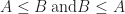


For example, we should require that:
[0, 1, 2]
[2, 0, 1]
And for two sequences which are not equal, like [0,1,2] and [3, 4, 5] we want the ordering to be invariant under permutation.
Obvious Solution
An obvious solution to this problem is to sort the arrays element-wise and return the result:
function compareSimple(a, b) {
  if(a.length !== b.length) {
    return a.length - b.length;
  }
  var as = a.slice(0)
    , bs = b.slice(0);
  as.sort();
  bs.sort();
  for(var i=0; i<a.length; ++i) {
    var d = as[i] - bs[i];
    if(d) {
      return d;
    }
  }
  return 0;
}
This follows the standard C/JavaScript convention for comparison operators, where it returns -1 if a comes before b, +1 if a comes after b and 0 if they are equal. For large enough sequences, this isn’t a bad solution. It takes 
An obvious way to fix this would be to try inlining the sorting function for small values of n (which is all we really care about), but doing this yourself is pure punishment. Here is an `optimized` version for length 2 sets:
function compare2Brutal(a, b) {
  if(a[0] < a[1]) {
    if(b[0] < b[1]) {
      if(a[0] === b[0]) {
        return a[1] - b[1];
      }
      return a[0] - b[0];
    } else {
      if(a[0] === b[1]) {
        return a[1] - b[0];
      }
      return a[0] - b[1];
    }
  } else {
    if(b[0] < b[1]) {
      if(a[1] === b[0]) {
        return a[0] - b[1];
      }
      return a[1] - b[0];
    } else {
      if(a[1] === b[1]) {
        return a[0] - b[0];
      }
      return a[1] - b[1];
    }
  }
}
If you have any aesthetic sensibility at all, then that code probably makes you want to vomit. And that’s just for length two arrays! You really don’t want to see what the version for length 3 arrays looks like. But it is faster by a wide margin. I ran a benchmark to try comparing how fast these two approaches were at sorting an array of 1000 randomly generated tuples, and here are the results:
- compareSimple: 5864 µs
- compareBrutal: 404 µs
That is a pretty good speed up, but it would be nice if there was a prettier way to do this.
Symmetry
The starting point for our next approach is the following screwy idea: what if we could find a hash function for each face that was invariant under permutations? Or even better, if the function was injective up to permutations, then we could just use the `symmetrized hash` compare two sets. At first this may seem like a tall order, but if you know a little algebra then there is an obvious way to do this; namely you can use the (elementary) symmetric polynomials. Here is how they are defined:
Given a collection of 


For example, if 


And for 


The neat thing about these functions is that they contain enough data to uniquely determine 
function compare2Sym(a, b) {
   var d = a[0] + a[1] - b[0] - b[1];
   if(d) {
     return d;
   }
   return a[0] * a[1] - b[0] * b[1];
}
Not only is this way shorter than the brutal method, but it also turns out to be a little bit faster. On the same test, I got:
- compare2Sym: 336 µs
Which is about a 25% improvement over brute force inlining. The same idea extends to higher n, for example here is the result for 
function compare3Sym(a, b) {
  var d = a[0] + a[1] + a[2] - b[0] - b[1] - b[2];
  if(d) {
    return d;
  }
  d = a[0] * a[1] + a[0] * a[2] + a[1] * a[2] - b[0] * b[1] - b[0] * b[2] - b[1] * b[2];
  if(d) {
    return d;
  }
  return a[0] * a[1] * a[2] - b[0] * b[1] * b[2];
}
Running the sort-1000-items test against the simple method gives the following results:
- compareSimple: 7637 µs
- compare3Sym: 352 µs
Computing Symmetric Polynomials
This is all well and good, and it avoids making a copy of the arrays like we used in the basic sorting method. However, it is also not very efficient. If one were to compute the coefficients of a symmetric polynomial directly using the naive method we just wrote, then you would quickly end up with 


A slightly better way to compute them is to use the polynomial formula and apply the FOIL method. That is, we just expand the symmetric polynomials using multiplication. This dynamic programming algorithm speeds up the time complexity to 
function compare3SymOpt(a,b) {
  var l0 = a[0] + a[1]
    , m0 = b[0] + b[1]
    , d  = l0 + a[2] - m0 - b[2];
  if(d) {
    return d;
  }
  var l1 = a[0] * a[1]
    , m1 = b[0] * b[1];
  d = l1 * a[2] - m1 * b[2];
  if(d) {
    return d;
  }
  return l0 * a[2] + l1 - m0 * b[2] - m1;
}
For comparison, the first version of compare3 used 11 adds and 10 multiplies, while this new version only uses 9 adds and 6 multiplies, and also has the option to early out more often. This may seem like an improvement, but it turns out that in practice the difference isn’t so great. Based on my experiments, the reordered version ends up taking about the same amount of time overall, more or less:
- compare3SymOpt: 356 µs
Which isn’t very good. Part of the reason for the discrepancy most likely has something to do with the way compare3Sym gets optimized. One possible explanation is that the expressions in compare3Sym might be easier to vectorize than those in compare3SymOpt, though I must admit this is pretty speculative.
But there is also a deeper question of can we do better than
Polynomial multiplication is convolution.
Using a fast convolution algorithm, we can multiply two polynomials together in 
Question: Can we compute the n elementary symmetric polynomials in
Overflow
Now there is still a small problem with using symmetric polynomials for this purpose: namely integer overflow. If you have any indices in your tuple that go over 1000 then you are going to run into this problem once you start multiplying them together. Fortunately, we can fix this problem by just working in a ring large enough to contain all our elements. In languages with unsigned 32-bit integers, the natural choice is 
But life is not so simple in the weird world of JavaScript! It turns out for reasons that can charitably be described as “arbitrary” JavaScript does not support a proper integer data type, and so every number type in the language gets promoted to a double when it overflows whether you like it or not (mostly not). The net result: the above approach messes up. One way to fix this is to try applying a modulus operator at each step, but the results are pretty bad. Here are the timings for a modified version of compare2Sym that enforces bounds:
- compare2Masked: 1750 µs
That’s more than a 5-fold increase in running time, all because we added a few innocent bit masks! How frustrating!
Semirings
The weirdness of JavaScript suggests that we need to find a better approach. But in the world of commutative rings, it doesn’t seem like there are any immediately good alternatives. And so we must cast the net wider. One interesting possibility is to extend our approach to include semirings. A semiring is basically a ring where we don’t require addition to be invertible, hence they are sometimes called “rigs” (which is short for a “ring without negatives”, get it? haha).
Just like a ring, a semiring is basically a set 


- The complex numbers are semiring (and more generally, so is every field)
- The integers are a semiring (and so is every other ring)
- The natural numbers are a semiring (but not a ring)
- The set of Boolean truth values,
under the operations OR, AND is a semiring (but is definitely not a ring)
- The set of reals under the operations min,max is a semiring (and more generally so is any distributive lattice)
- The tropical semiring, which is the set of reals under (max, +) is a semiring.
In many ways, semirings are more fundamental than rings. After all, we learn to count stuff using the natural numbers long before we learn about integers. But they are also much more diverse, and some of our favorite definitions from ring theory don’t necessarily translate well. For those who are familiar with algebra, probably the most shocking thing is that the concept of an ideal in a ring does not really have a good analogue in the language of semirings, much like how monoids don’t really have any workable generalization of a normal subgroup.
Symmetric Polynomials in Semirings
However, for the modest purposes of this blog post, the most important thing is that we can define polynomials in a semiring (just like we do in a ring) and that we therefore have a good notion of an elementary symmetric polynomial. The way this works is pretty much the same as before:
Let 


And for


And so on on…
Rank Functions and (min,max)
Let’s look at what happens if we fix a particular semiring, say the (min,max) lattice. This is a semiring over the extended real line 


Now, here is a neat puzzle:
Question: What are the elementary symmetric polynomials in this semiring?
Here is a hint:


And…

Give up? These are the rank functions!
Theorem: Over the min,max semiring,

In other words, evaluating the symmetric polynomials over the min/max semiring is the same thing as sorting. It also suggests a more streamlined way to do the brutal inlining of a sort:
function compare2Rank(a, b) {
  var d = Math.min(a[0],a[1]) - Math.min(b[0],b[1]);
  if(d) {
    return d;
  }
  return Math.max(a[0],a[1]) - Math.max(b[0],b[1]);
}
Slick! We went from 25 lines down to just 5. Unfortunately, this approach is a bit less efficient since it does the comparison between a and b twice, a fact which is reflected in the timing measurements:
- compare2Rank: 495 µs
And we can also easily extend this technique to triples as well:
function compare3Rank(a,b) {
  var l0 = Math.min(a[0], a[1])
    , m0 = Math.min(b[0], b[1])
    , d  = Math.min(l0, a[2]) - Math.min(m0, b[2]);
  if(d) {
    return d;
  }
  var l1 = Math.max(a[0], a[1])
    , m1 = Math.max(b[0], b[1]);
  d = Math.max(l1, a[2]) - Math.max(m1, b[2]);
  if(d) {
    return d;
  }
  return Math.min(Math.max(l0, a[2]), l1) - Math.min(Math.max(m0, b[2]), m1);
}
- compare3Rank: 618.71 microseconds
The Tropical Alternative
Using rank functions to sort the elements turns out to be much simpler than doing a selection sort, and it is way faster than calling the native JS sort on small arrays while avoiding the overflow problems of integer symmetric functions. However, it is still quite a bit slower than the integer approach.
The final method which I will now describe (and the one which I believe to be best suited to the vagaries of JS) is to compute the symmetric functions over the (max,+), or tropical semiring. It is basically a semiring over the half-extended real line, 


There is a cute story for why the tropical semiring has such a colorful name, which is that it was popularized at an algebraic geometry conference in Brazil. Of course people have known about (max,+) for quite some time before that and most of the pioneering research into it was done by the mathematician Victor P. Maslov in the 50s. The (max,+) semiring is actually quite interesting and plays an important role in the algebra of distance transforms, numerical optimization and the transition from quantum systems to classical systems.
This is because the (max,+) semiring works in many ways like the large scale limit of the complex numbers under addition and multiplication. For example, we all know that:

But did you also know that:

This basically a formalization of that time honored engineering philosophy that once your numbers get big enough, you can start to think about them on a log scale. If you do this systematically, then you eventually will end up doing arithmetic in the (max,+)-semiring. Masolv asserts that this is essentially what happens in quantum mechanics when we go from small isolated systems to very big things. A brief overview of this philosophy that has been translated to English can be found here:
Litvinov, G. “The Maslov dequantization, idempotent and tropical mathematics: a very brief introduction” (2006) arXiv:math/0501038
The more detailed explanations of this are unfortunately all store in thick, inscrutable Russian text books (but you can find an English translation if you look hard enough):
Maslov, V. P.; Fedoriuk, M. V. “Semiclassical approximation in quantum mechanics”
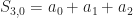
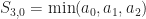
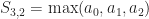
But enough of that digression! Let’s apply (max,+) to the problem at hand of comparing sequences. If we expand the symmetric polynomials in the (max,+) world, here is what we get:


And for


If you stare at this enough, I am sure you can spot the pattern:
Theorem: The elementary symmetric polynomials on the (max,+) semiring are the partial sums of the sorted sequence.
This means that if we want to compute the (max,+) symmetric polynomials, we can do it in
Working the (max,+) solves most of our woes about overflow, since adding numbers is much less likely to go beyond INT_MAX. However, we will tweak just one thing: instead of using max, we’ll flip it around and use min so that the values stay small. Both theoretically and practically, it doesn’t save much but it gives us a maybe a fraction of a bit of extra address space to use for indices. Here is an implementation for pairs:
function compare2MinP(a, b) {
  var d = a[0]+a[1]-b[0]-b[1];
  if(d) {
    return d;
  }
  return Math.min(a[0],a[1]) - Math.min(b[0],b[1]);
}
And it clocks in at:
- compare2MinP: 354 µs
Which is a bit slower than the symmetric functions, but still way faster than ranking. We can also play the same game for
function compare3MinP(a, b) {
  var l1 = a[0]+a[1]
    , m1 = b[0]+b[1];
  d = l1+a[2] - (m1+b[2]);
  if(d) {
    return d;
  }
  var l0 = Math.min(a[0], a[1])
    , m0 = Math.min(b[0], b[1])
    , d  = Math.min(l0, a[2]) - Math.min(m0, b[2]);
  if(d) {
    return d;
  }
  return Math.min(l0+a[2], l1) - Math.min(m0+b[2], m1);
}
Which hits:
- compare3MinP: 382 µs
Again, not quite as fast as integers, but pretty good for JavaScript.
Summary
You can get all the code to run these experiments on github:
https://github.com/mikolalysenko/set-compare
And here are the results that I got from running the experiment, all collated for easy reading:
Dimension = 2
- compareSimple: 5982 µs
- compare2Brutal: 415 µs
- compare2Sym: 352 µs
- compare2SymMasked: 1737 µs
- compare2Rank: 498 µs
- compare2MinP: 369 µs
Dimension = 3
- compareSimple: 7737 µs
- compare3Sym: 361 µs
- compare3Sym_opt: 362 µs
- compare3Rank: 612 µs
- compare3MinP: 377 µs
As you can see, the (min,+) solution is nearly as fast as the symmetric version without having the same overflow problems.
I hope you enjoyed reading this as much as I enjoyed tinkering around! Of course I still don’t know of an optimal way to compare two lists. As a final puzzle, I leave you with the following:
Question: Is there any method which can test if two unordered sequences are equal in linear time and at most log space?
Frankly, I don’t know the answer to this question and it may very well be impossible. If you have any thoughts or opinions on this, please leave a comment!

 . As we have already seen, it is possible to
  where
where  . Then we can define our shape as the preimage of some subset of these labels,
  :
:
 and
and ![S_0 = (-\infty, 0]](https://s0.wp.com/latex.php?latex=S_0+%3D+%28-%5Cinfty%2C+0%5D&bg=ffffff&fg=1a1a1a&s=0&c=20201002) , then we get the usual definition of a sublevel set:
, then we get the usual definition of a sublevel set:
 of truth values, and we might consider defining our shape as the preimage of 1:
 to warp it into a new position:
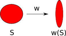
 and we have some warp
  is the 0-sublevel set of some potential function
  , can we find another potential function
  such that,
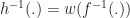

 is invertible. So in summary,
 by
by 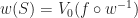

![[0,1]](https://s0.wp.com/latex.php?latex=%5B0%2C1%5D&bg=ffffff&fg=1a1a1a&s=0&c=20201002) ) into some ambient space, say
) into some ambient space, say 

 be a parameterization of a shape
