Large voxel terrains may contain millions of polygons. Rendering such terrains at a uniform scale is both inefficient and can lead to aliasing of distant objects. As a result, many game engines choose to implement some form of level of detail based rendering, so that distant terrain is rendered with less geometry.
In this post, I’ll talk about a simple technique based on vertex clustering with some optimizations to improve seam handling. The specific ideas in this article are applied to Minecraft-like blocky terrain using the same clustering/sorting scheme as POP buffers.
Progressively Ordered Primitive (POP) buffers are a special case of vertex clustering, where for each level of detail we round the vertices down to the previous power of two. The cool thing about them is that unlike other level of detail methods, they are implicit, which means that we don’t have to store multiple meshes for each level detail on the GPU.
When any two vertices of a cell are rounded to the same point (in other words, an edge collapse), then we delete that cell from that level of detail. This can be illustrated in the following diagram:
Suppose that each vertex has integer coordinates. Define,
Each of the sets represents the topology mesh at some level of detail, with being the finest, full detail mesh and the coarsest. To get the actual geometry at level , we can take any and compute,
Using this property, we can encode the different levels of detail by sorting the primitives of the mesh from coarse-to-fine and storing a table of offsets:
To render the mesh at any level of detail we can adjust the vertex count, and round the vertices in the shader.
Building POP buffers
To construct the POP buffer, we need to sort the quads and count how many quads are in each LOD. This is an ideal place to use counting sort, which we can do in-place in O(n) time, illustrated in the following psuedo-code:
// Assume MAX_LOD is the total number of levels of detail
// quadLOD(...) computes the level of detail for a quad
function sortByLOD (quads) {
    const buckets = (new Array(MAX_LOD)).fill(0)
    // count number of quads in each LOD
    for (let i = 0; i < quads.length; ++i) {
        buckets[quadLOD(quads[i])] += 1
    }
    // compute prefix sum
    let t = 0;
    for (let i = 0; i < MAX_LOD; ++i) {
       const b = buckets[i]
       buckets[i] = t
       t += b
    }
    // partition quads across each LOD
    for (let i = quads.length - 1; i >= 0; --i) {
        while (true) {
            const q = quads[i]
            const lod = quadLOD(q)
            const ptr = buckets[lod]
            if (i < ptr) {
                break;
            }
            quads[i] = quads[ptr]
            quads[ptr] = q
            buckets[lod] += 1
        }
    }
    // buckets now contains the prefixes for each LOD
    return buckets
}
The quadLOD() helper function returns the coarsest level of detail where a quad is non-degenerate. If each quad is an integer unit square (i.e. not the output from a greedy mesh), then we can take the smallest corner and compute the quad LOD in constant time using a call to count-trailing zeroes. For general quads, the situation is a bit more involved.
LOD computation
For a general axis-aligned quad, we can compute the level of detail by taking the minimum level of detail along each axis. So it then suffices to consider the case of one interval, where the level of detail can be computed by brute force using the following algorithm:
function intervalLOD (lo, hi) {
    for (let i = 0; i <= 32; ++i) {
        if ((lo >> i) === (hi >> i)) {
            return i
        }
    }
}
We can simplify this if our platform supports a fast count-leading-zeroes operation:
function intervalLOD (lo, hi) {
    return countLeadingZeroes(lo ^ hi)
}
Squashed faces
The last thing to consider is that when we are collapsing faces we can end up with over drawing due to rounding multiple faces to the same level. We can remove these squashed faces by doing one final pass over the face array and moving these squashed faces up to the next level of detail. This step is not required but can improve performance if the rendering is fragment processing limited.
Geomorphing, seams and stable rounding
In a voxel engine we need to handle level of detail transitions between adjacent chunks. Transitions occur when we switch from one level of detail to another abruptly, giving a discontinuity. These can edges be hidden using skirts or transition seams at the expense of greater implementation complexity or increased drawing overhead.
In POP buffers, we can avoid the discontinuity by making the level of detail transition continuous, similar to 2D terrain techniques like ClipMaps or CLOD. Observe that we can interpolate between two levels of detail using vertex morphing,
In the original POP buffer paper, they proposed a simple logarithmic model for selecting the LOD parameter as a function of the vertex coordinate :
Where is a bias parameter (based on the display resolution, FOV and hardware requirements) and viewDist is a function that computes the distance to the vertex from the camera. Unfortunately, this LOD function is discontinuous across gaps due to rounding.
The authors of the original POP buffer paper proposed modifying their algorithm to place vertices along the boundary at the lowest level of detail. This removes any cracks in the geometry, but increases LOD generation time and the size of the geometry.
Instead we can solve this problem using a stable version of LOD rounding. Let be the maximum LOD value for the chunk and all its neighbors. Then we compute a fixed point for :
In practice 2-3 iterations is usually sufficient to get a stable solution for most vertices. This iteration can be implemented in a vertex shader and unrolled, giving a fast seamless level of detail selection.
As an aside, this construction seems fairly generic. The moral of the story is really that if we have geomorphing, then we don’t need to implement seams or skirts to get crack-free LOD.
World space texture coordinates
Finally, the last issue we need to think about are texture coordinates. We can reuse the same texturing idea from greedy meshing. For more info see the previous post.
Been a long time since I’ve written anything here. Lately I’ve been working on a new multiplayer WebGL voxel engine for codemao (an educational platform to teach kids programming via games). It’s not live yet, but a bunch of neat ideas have come out of this project. In this post I want to talk about the lighting model and share some of the tricks which were used to speed up processing.
Conceptually the basic lighting system is similar to the one used in Minecraft and Seed of Andromeda with a few small tweaks. For background information, I would recommend the following sources:
This post describes some extensions and optimizations to the basic flood fill lighting model proposed by Ben Arnold. In particular, we show how to adapt ambient occlusion to track a moving sun, and how to improve flood fill performance using word-level parallelism bit tricks.
Recap of flood fill lighting
Flood fill lighting is an approximation of ambient occlusion where lighting values are propagated using a breadth-first search along the 6-faces of each cube. To the best of my knowledge, Minecraft is the first game to use technique to approximate global illumination, but Ben Arnold is the first to write about it in detail. Minecraft tracks two separate lighting channels. One for global light values based on time of day, and one for block light levels derived from objects like torches. This allows for the color of the day light to change dynamically without requiring large terrain updates. Ben Arnold improves on this basic pattern by storing a separate light level for the red/green/blue allowing for colored light sources:
Minecraft: 1 byte = 4 bits for torch light + 4 bits for sky light
Seed of andromeda: 2 bytes = 4 bits red + 4 bits green + 4 bits blue + 4 bits sky
This post: 4 bytes = 4 bits red + 4 bits green + 4 bits blue + 5 * 4 bits sky
Multidirectional sun light
The first improvement we propose in this model is modifying the sky light to support multiple directions. Instead of sampling only sunlight propagation along the y-axis, we also sample along the +/-x axes and the 45-degree diagonal x-y lines and compute ambient contributions for these angle independently:
This requires storing 4 extra light coefficients per-voxel, and if we use 4-bits per coefficient, then this is a total of 16 extra bits. Combined with the previous 16-bits, this means we need 32-bits of extra lighting data per voxel.
To track the lighting values for the other axes we do essentially the same thing for each extra component. In the case of the +/-x axes, it should be clear enough how this works. For the diagonal axes we can trace through a sheared volume. To index into the diagonal textures we take either the sum/ difference of the x and y components and to get the distance along the ray we can just use the y-value.
Word level parallelism
When propagating light field, we need to often perform component-wise operations on the channels of each light field, which we can pack into a single machine word. Here’s a picture of how this looks assuming 4-bits per channel for the simpler case of a 32-bit value:
We could do operations on each channel using bit masking/shifting and looping, however there is a better way: word level parallelism. We’ll use a general pattern of splitting the coefficients in half and masking out the even/odd components separately so we have some extra space to work. This can be done by bit-wise &’ing with the mask 0xf0f0f0f:
Less than
The first operation we’ll consider is a pair-wise less than operation. We want to compare two sets of lighting values and determine which components are < the other. In pseudo-JS we might implement this operation in the following naive way:
function lightLessThan (a, b) {
 let r = 0;
 for (let i = 0; i < 8; ++i) {
   if ((a & (0xf << i)) < (b & (0xf << i))) {
     r |= 0xf << i;
   }
 }
 return r;
}
We can avoid this unnecessary looping using word-level parallelism. The basic idea is to subtract each component and use the carry flag to check if the difference of each component is negative. To prevent underflow we can bitwise-or in a guard so that the carry bits are localized to each component. Here’s a diagram showing how this works:
Putting it all together we get the following psuedo-code:
Building on this we can find component-wise maximum of two light vectors (necessary when we are propagating light values). This key idea is to use the in place bit-swap trick from the identity:
Combined with the above, we can write component-wise max as:
function wlpMax (a, b) {
 return a ^ ((a ^ b) & wlpLT(a, b));
}
Decrement-and-saturate
Finally, in flood fill lighting the light level of each voxel decreases by 1 as we propagate. We can implement a component-wise-decrement and saturate again using the same idea:
function wlpDecHalf (x) {
 // compute component-wise decrement
 const d = ((x & 0xf0f0f0f) | 0x20202020) - 0x1010101;

// check for underflow
 const b = d & 0x10101010;

// saturate underflowed values
 return (d + (b >> 4)) & 0x0f0f0f0f;
}

// decrement then saturate each 4 bit component of x
function wlpDec (x) {
 return wlpDecHalf(x) | (wlpDecHalf(x >> 4) << 4);
}
It has been a while since I’ve written about Minecraft-like games, and so today I figured I’d take a moment to discuss something which seems to come up a lot in online discussions, specifically how to implement ambient occlusion in a Minecraft-like game:
Smooth lighting in Minecraft. (c) Mojang AB. Image obtained from Minecraft wiki.
Ambient occlusion was originally introduced into Minecraft as a mod, and eventually incorporated into the core Minecraft engine along with a host of other lighting improvements under the general name of “smooth lighting”. To those who are in-the-know on voxel engine development, this stuff is all pretty standard, but I haven’t yet seen it written up in an accessible format yet. So I decided to write a quick blog post on it, as well as discuss a few of the small technical issues that come up when you implement it within a system that uses greedy meshing.
Ambient Occlusion
Ambient occlusion is a simple and effective technique for improving the quality of lighting in virtual environments. The basic idea is to approximate the amount of ambient light that is propagated through the scene towards a point from distant reflections. The basis for this idea is a heuristic or empirical argument, and can be computed by finding the amount of surface area on a hemisphere which is visible from a given point:
Adding an ambient occlusion factor to a scene can greatly improve the visual fidelity, and so a lot of thought has gone into methods for calculating and approximating ambient occlusion efficiently. Broadly speaking, there are two general approaches to accessibility computation:
Static algorithms: Which try to precalculate ambient occlusion for geometry up front
Dynamic algorithms: Which try to compute accessibility from changing or dynamic data.
Perhaps the most well known of these approaches is the famous screen-space ambient occlusion algorithm:
The general idea is to read out the contents of the depth buffer, and then use this geometry to approximate the accessibility of each pixel. This can then be used to shade all of the pixels on the screen:
Screen space ambient occlusion for a typical game. Public domain. Credit: Vlad3D.
Screen space ambient occlusion is nice in that it is really easy to integrate into an existing rendering pipeline — especially with deferred shading — (it is just a post process!) but the downside is that because the depth buffer is not a true model of the scene geometry it can introduce many weird artefacts. This link has a brief (humorous/NSFW) survey of these flaws.
Ambient occlusion for voxels
Fortunately, in a voxel game there is a way to implement ambient occlusion which is not only faster, but also view independent. The general idea is to calculate the ambient occlusion for each vertex using only the information from the cubes which are adjacent to it. Taking this into account, there are up to symmetry 4 possible ambient occlusion values for a vertex:
The four different cases for voxel ambient occlusion for a single vertex.
Using this chart we can deduce a pattern. Let side1 and side2 be 0/1 depending on the presence of the side voxels and let corner be the opacity state of the corner voxel. Then we can compute the ambient occlusion of a vertex using the following function:
It is actually quite easy to integrate the above ambient occlusion algorithm into a system that uses greedy meshing. The key idea is that we just need to merge facets which have the same ambient occlusion value across each of their vertices. This works because along each of the greedy edges that have length greater than 1 voxel the ambient occlusion values of the greedy mesh will be constant (exercise for reader: prove this). So, there is almost nothing to do here except modify the code that checks if two voxels should be merged.
There is a second issue here though that is a bit more subtle. Recall that to render a quad on it needs to be subdivided into two triangles. This subdivision introduces anisotropy in how non-linear values will get interpolated along a quad. For the case where the ambient occlusion values of a quad are not coplanar, this will introduce a dependence on how the quad is subdivided. To illustrate this effect, consider the following picture:
Errors in ambient occlusion shading due to anisotropy.
Notice that the ambient occlusion is different for the vertices on the side than it is for the vertices on the top and bottom. To fix this, we just need to pick a consistent orientation for the quads. This can be done by comparing the ambient occlusion terms for each quad and selecting an appropriate orientation. Supposing that a00, a01, a11, a01 are the ambient occlusion values for the four vertices of a quad sorted in clockwise order. Then we can correct this problem using the following rule:
This one simple trick easily fixes the display problem:
Correctly shaded ambient occlusion. Note that all four vertices are rendered the same.
Conclusion
Adding ambient occlusion to a voxel game is super easy to do and carries little cost besides a modest increase in mesh construction time. It also improves the visual quality of the results enormously, and so it is one of those no-brainer features to add. There are plenty of places to go further with this. For example, you could take the ambient occlusion of the complement space to create translucency effects in a voxel game (kind of like this idea). You would also probably want to combine this technique with other more sophisticated lighting methods to handle things like shadows and possibly reflections, but this maybe a better topic for another post.
EDIT 1: Embarrassingly I had the initial definition for ambient occlusion wrong. I fixed this.
EDIT 2: Mrmessiah, whois probably the true inventor of this technique commented on a reddit thread about this and said the following:
This post caught my eye – I was the guy that wrote the original Ambient Occlusion mod for Minecraft. Minecraft’s original lighting system (I think!) had air blocks with discrete lighting levels from 0 to 15 and any block face exposed to one took its lighting level from that.
You sum it up how the first working version of my algorithm worked pretty well! That first version still had the “blocky” look because the underlying faces were still taking their light level from the air block touching them, but at least the AO effect softened it a bit where you had geometry nearby. editHere’s the very first pic of it working on my test map and you can see what I mean about the “blocky light with AO” thing.
The smooth lighting variant came later – that worked slightly differently, by averaging light levels at vertices on a plane. Originally I had thought I would have that as an “additional” effect on top of the AO effect, and just apply it on flat surfaces. But then I realised, because the lighting level of solid blocks was 0, I could just do that averaging everywhere, and it’d give me AO for free. I suck at explaining without diagrams, unfortunately. 😦
I should say that the lighting system currently in Minecraft was written by Jeb, he did contact me to see about using mine and I said “sure” and offered to give him my code but I think he reimplemented his own variant of it in the mean time.
Don’t know if I was the first person to come up with either algorithm, but it was fun working out how to do it.
EDIT 3: Since posting this, I’ve learned about at least two other write ups of this idea. Here they are:
Continuing in the recreational spirit of this blog, this week I want to write about something purely fun. In particular, I’m going to tell you how to convert retro 16 x 16 sprites into 3D miniatures:
Turning an 8-bit sprite into a 3D model
This project was motivated purely by intellectual curiosity, and doesn’t really have too many practical application. But it is pretty fun, and makes some neat looking pictures. There is also some very beautiful math behind it, which I’ll now explain:
From 2D to 3D
It is a fundamental problem in computer vision to turn a collection of 2D images into a 3D model. There are a number of ways to formulate this problem, but for this article I am going to focus on the following specialization of the problem which is known as multiview stereo reconstruction:
Given a collection of images of an unknown static object under known viewing configurations and lighting conditions, reconstruct the 3D object.
There are a few things about this which may seem a bit contrived; for example we might not always know where the camera is and what the lighting/material properties are like; however this are a still a large number of physical systems capable of taking these sort of controlled measurements. One famous device is the Stanford spherical gantry, which can take photos of an object from points on a spherical shell surrounding. In fact, this machine has been used to produce a number of famous datasets like the well known “Dino” and “Temple” models:
One of the images from the temple data set acquired by the Stanford spherical gantry.
Of course even with such nice data, the multiview stereo problem is still ill-posed. It is completely possible that more than one possible object might be a valid reconstruction. When faced with such an ill posed problem, the obvious thing to do would be to cook up some form statistical model and apply Bayesian reasoning to infer something about the missing data. This process is typically formulated as some kind of expectation maximization problem, and is usually solved using some form of non-linear optimization process. While Bayesian methods are clearly the right thing to do from a theoretical perspective; and they have also been demonstrated to be extremely effective at solving the 3D reconstruction problem in practice, they are also incredibly nasty. Realisitic Bayesian models, (like the ones used in this software, for example), have enormous complexity, and typically require many hand picked tuning parameters to get acceptable performance.
Photo Hulls
All of this machine learning is quite well and good, but it is way too much overkill for our simple problem of reconstructing volumetric graphics from 8-bit sprites. Instead, to make our lives easier we’ll use a much simpler method called space carving:
UPDATE: After Chuck Dyer’s comment, I now realize that this is probably not the best reference to cite. In fact, a better choice is probably this one, which is closer to what we are doing here and has priority by at least a year:
(In fact, I should have known this since I took the computer vision course at UW where Prof Dyer works. Boy is my face red!) /UPDATE
While space carving is quite far from being the most accurate multiview stereo algorithm, it is still noteworthy due to its astonishing simplicity and the fact that it is such a radical departure from conventional stereo matching algorithms. The underlying idea behind space carving is to reformulate the multiview stereo matching problem as a fairly simple geometry problem:
Problem: Given a collection of images at known configurations, find the largest possible object in a given compact region which is visually consistent with each view.
If you see a crazy definition like this, the first thing you’d want to know is if this is even well-defined. It turns out that the answer is “yes” for suitable definitions of “visually consistent”. That is, we require that our consistency check satisfy few axioms:
Ray Casting: The consistency of a point on the surface depends only on the value of the image of each view in which it is not occluded.
Monotonicity: If a point is consistent with a set of views , then it is also consistent with any subset of the views .
Non-Triviality: If a point is not visibile in any view, then it is automatically consistent.
It turns out that this is true for almost any reasonable definition of visual consistency. In particular, if we suppose that our object has some predetermined material properties (ie is Lambertian and non-transparent) and that all our lighting is fixed, then we can check consistency by just rendering our object from each view and comparing the images pixel-by-pixel. In fact, we can even say something more:
Photo-Hull Theorem (Kutulakos & Seitz): The solution to the above problem is unique and is the union of all objects which are visually consistent with the views.
Kutulakos and Seitz call this object the photo hull of the images, by an analogy to the convex hull of a point set. The photo hull is always a super set of the actual object, as illustrated in Fig. 3 of the above paper:
The photo hull illustrated. On the left is the physical configuration of an object and several cameras placed around it. On the right is the reconstructed photohull of the object. Note that both the left and right object produce identical projections. (c) 2000 Kutulakos&Seitz
If you stare at the above picture enough, and try looking at some of the examples in that paper you should get a pretty good idea of what the photo hull does. Once you have some intuition for what is going here, it is incredibly simple to prove the above theorem:
Proof: It suffices to show that the photo hull, , is visually consistent. So suppose by contradiction that it is not; then there exists some point . But by definition, there must be some visually consistent set containing . However, since is a strict subset, the number views in which is visible is a super set of the views containing it in , and so by monotonicity and locality can not be visually consistent. Therefore, is photo consistent and its uniqueness follows from the boundedness of the containing region.
Carving Out Sprites
So now that we know what a photo hull is and that it exists, let’s try to figure out how to compute it. It turns out that the above proof is highly suggestive of an algorithm. What you could do is start with some large super set containing the object, then iteratively carve away inconsistent bits of the region until all you are left with is the maximal visually consistent set; or in other words the photo hull. One simple way to accomplish this is to suppose that our region is really a voxel grid and then do this carving by a series of plane sweeps, which is essentially what Kutulakos and Seitz describe in their paper.
To make all of this concrete, let’s apply it to our problem of carving out voxel sprites. The first thing we need to do is figure out what material/lighting model to use. Because we are focusing on retro/8-bit sprites, let us make the following assumption:
Flat Lighting Model: Assume that the color of each voxel is contant in each view.
While this is clearly unphysical, it actually applies pretty well to sprite artwork, especially those drawn using a limited pallet. The next thing we need to do is pick a collection of viewing configurations to look at the sprite. To keep things simple, let us suppose that we view each sprite directly along the 6 cardinal directions (ie top, bottom, front, back, left, right) and that our cameras are all orthographic projections:
Putting this all together with the above sweep line method gives us a pretty simple way to edit sprites directly
Filling in the Gaps
Of course there is still one small problem. The shape we get at the end may have some small gaps that were not visible in any of the 6 views and so they could not be reconstructed. To get a decent looking reconstruction, we have to do something about these missing points. One simple strategy is to start from the edges of all these holes and then work inwards, filling in the missing pixels according to the most frequently occuring colors around their neighbors. This produces pretty good results for most simple sprites, for example:
Left: No in painting. Right: With in painting
Unfortunately, the limitations become a bit more apparent near regions when the image has some texture or pattern:
Left: No in painting. Right: With in painting. Note that the patterns on the left side are not correctly matched:
A better model would probably be to using something like a Markov random field to model the distribution of colors, but this simple mode selection gives acceptable results for now.
Editor Demo
As usual, I put together a little WebGL demo based on this technique. Because there isn’t much to compare in this experiment, I decided to try something a bit different and made a nifty interactive voxel editor based on these techniques. You can try it out here:
Here is a break down of the user interface for the editor:
And here is what all the buttons do:
3D View: This is a 3D view of the photo hull of your object. To move the viewing area around, left click rotates, middle click zooms and right click pans. Alternatively, if you are on a mac, you can also use “A”, “S”, “D” to rotate/zoom/pan.
Fill Hidden: If you want to see what it looks like without the “gap filling” you can try unchecking the “Fill Hidden” feature.
Sprite Editors: On the upper left side of the screen are the editor panes. These let you edit the sprites pixel-by-pixel. Notice that when you move your cursor around on the editor panes, it draws a little red guide box showing you what subset of the model will be affected by changing the given pixel.
Show Guides: If the guide boxes annoy you, you can turn them off by deselecting “Show Guides” option.
Paint Color: This changes the color for drawing, you can click on the color picker at the bottom of the editor. There is also an “eye dropper” feature to select another color on the sprite, where if you middle/shift click on a pixel in the sprite editor, then it will set the paint color to whatever you have highlighted. Note that black (or “#000000”) means “Do not fill”.
Palette: To simplify editing sprite art, there is also a palette feature on the page. You can set the paint color to a palette color by clicking on your palette; or you can save your paint color to the palette by shift/middle clicking on one of the palette items.
Reconstruct Selected Views: You can use this feature to automatically reconstruct some of the views of the object. To select the views, click the check boxes (7a) and then to fill them in click “Reconstruct Selected Views” (7b). This can be helpful when first creating a new object.
Import Image: Of course if editing images in a web browser is not your cup of tea, you can easily export your models and work offline (using tools like MSPaint or Photoshop) and then upload them to the browser when you are done. The “Import Image” button lets you save the shape you are currently working on so you can process it offline.
Export Image: The “Export Image” button is the dual of the dual of “Import Image” and lets you take images you built locally and upload them to the server for later processing.
Share: This button lets you share your model online. When you click it, a link will show up once your model has been uploaded to the server, which you can then send to others.
Print in 3D: This button uploads your model to ShapeWays so you can buy a 3D miniature version of your model in real life (more below).
There are also some more advanced features:
Undo: To undo the last action, press Ctrl+Z
Eye Dropper: To select a color on the sprite, you can either shift/alt/ctrl/middle/right click a color on the sprite editor.
Save to Palette: To save your current paint color to the palette, you can shift/alt/ctrl/middle/right click a palette entry.
Screenshot: To take a screen shot of your model, press “p”
Fullscreen: “f” toggles fullscreen mode
Pan/Zoom: Middle click or holding “s” zooms in and out. Right click or holding “d” pans the camera.
Inconsistent Pixels: Are highlighted in magenta on the sprite editor pane.
Sweep Preview: Selecting views in the sprite editor filters them from the 3d object.
The source code for the client is available on GitHub, so feel free to download it and try it out. (Though be warned! The code is pretty ugly!) Also please post any cool stuff you make in the comments!
3D Printing
The last cool thing that I added was the ability to 3D print your models on the ShapeWays store once you are done. This means that you can take your designs and turn them into nifty 3D miniatures:
A 3D printed miniature.
The resulting miniatures are about 5cm or 2in tall, and are super cool. You can also look at the gallery of all the stuff everyone has uploaded so far on ShapeWays at the official store:
For every object that gets printed using this service, $10 gets donated to help support this blog. If this fee is too expensive for you, the client is open source and you can basically copy the models out of the browser and print them yourself. However, if you like the content on this site and want to help out, then please consider making a $10 donation by ordering a printed miniature through the store interface. Not only will you be helping out, but you’ll also get a cool toy as well!
Acknowledgements
Thanks to everyone on facebook and #reddit-gamedev for early feedback. Also, thanks to ShapeWays for providing the 3D printing service. The client uses three.js for rendering and jsColor for color picking. The backend is written in node.js using mongodb, and relies on ShapeWays.JS to interface with ShapeWays’ service. Mario and Link are both copyrighted by Nintendo. MeatBoy is copyrighted by Team Meat. Please don’t sue me!
To briefly recap, our goal is to render large volumetric environments. For the sake of both efficiency and image quality, we want to introduce some form of level of detail simplification for distant geometry. Last time, we discussed two general approaches to level of detail — surface and volumetric — focusing primarily on the former. Though volumetric terrain is not exactly the same as height-map based terrain, we can draw an imperfect analogy between these two problems and the two most popular techniques for 2D terrain rendering: ROAM and geometry clipmaps.
ROAM vs. Clip Maps
ROAM, or Realtime Optimally Adapting Meshes, is in many ways the height-field equivalent of surface based simplification. In fact, ROAM is secretly just the simplification envelopes algorithm applied to large regular grids! For any viewing configuration and triangle budget, ROAM computes an optimally simplified mesh in this sense. This mesh is basically as good as it gets, modulo some twiddle factors with the error metric. The fact that ROAM produces nicely optimized meshes made it very popular in the late nineties — an era when rasterization was much more expensive than GPU bandwidth.
The downside to ROAM is that when your camera moves, this finely tuned mesh needs to be recalculated (though the changes may not be too big if your camera motion is small enough). The cost of these updates means that you need to send a lot of geometry and draw calls down the GPU pipeline each frame, and that your CPU has to burn many cycles recalculating and updating the mesh. Though the approach of “build the best mesh possible” once made a lot of sense, as GPUs got faster and faster, eventually leaving CPUs in the dust, the rasterization vs bandwidth tradeoff shifted dramatically in the other direction, eventually making other strategies more competitive.
Geometry clipmaps are the modern replacement for ROAM, and are designed with the reality of GPU hardware in mind. Instead of trying to fully optimize the terrain mesh, clipmaps instead approximate different levels of detail by resampling the heightfield. That is, at all levels of detail the terrain mesh is always rendered as a uniform grid, it’s just that as we go farther away from the camera it becomes less dense. While geometry clipmaps produce lower quality meshes than ROAM, they make up for this short-coming by using much less GPU bandwidth. The clever idea behind this technique is to update the different levels of detail using a rolling hierarchy of toroidal buffers. This technique was first described in the following paper:
The first mention of using clipmaps for GPU accelerated terrain appears to be an old article on flipcode by Willem de Boer from late 2000 — though the credit for popularizing the idea usually goes to the following two papers, which rediscovered the technique some years later:
In practice, clipmaps turn out to be much faster than ROAM for rendering large terrains at higher qualities. In fact, clipmaps have been so successful for terrain rendering that today the use of ROAM has all but vanished. I don’t think too many graphics programmers lament its obsolescence. ROAM was a lot more complicated, and had a bad reputation for being very difficult to implement and debug. Clipmaps on the other hand are simple enough that you can get a basic implementation up and running in a single sitting (assuming you already have a decent graphics framework to start from).
Clipmaps for Isosurfaces
Given that clipmaps work so well for heightfields, it seems intuitive that the same approach might work for large isosurfaces as well. Indeed, I am aware of at least a couple of different attempts to do this, but they are all somewhat obscure and poorly documented:
Genova Terrain Engine: As far as I know, Peter Venis’ Genova terrain engine is one of the first programs capable of rendering large volumetric terrain in real time. What is more impressive is that it did all of this in real-time back in 2001 on commodity graphics hardware! During the time when flipcode was still active, this project was quite famous:
Screenshot of the Genova terrain engine, recovered from the Internet Archive. (c) Peter Venis 2001
Unfortunately, there is not much information available on this project. The original website is now defunct, and the author appears to have vanished off the face of the internet, leaving little written down. All that remains are a few pages left in the internet archive, and some screenshots. However, from what little information we do have, we could draw a few probable conclusions:
Genova probably uses surface nets to extract the isosurface mesh.
It also supports some form of level of detail, probably volumetric.
Internally it uses some form of lossless compression (probably run-length encoding).
Beyond that, it is difficult to say much else. It is quite a shame that the author never published these results, as it would be interesting to learn how Genova actually works.
UPDATE: I receive an email from Peter saying that he has put the website for Project Genova back online and that the correct name for the project is now Genova. He also says that he has written another volumetric terrain engine in the intervening years, so stay tuned to see what else he has in store.
HVox Terrain Engine: Sven Forstmann has been active on flipcode and gamedev.net for many years, and created several voxel rendering engines. In particular, his HVox engine, that he released way back in 2004 is quite interesting:
Sven Forstmann’s HVox engine, circa 2004. Image (c) Sven Forstmann.
It is hard to find details about this algorithm, but at least it seems like some stuff did ultimately get written up about it (though it is not easily accessible). Like the Genova terrain engine, it seems that HVox uses some combination of surface nets and geometry clip maps, though I am not fully confident about this point. The major details seem to be contained in an unpublished technical report, that I can’t figure out how to download. (If anyone out there can get a copy or knows how to contact Forstmann, I’d love to read what he has written.) In the end, I suspect that some of the technology here may be similar to Genova, but as the details about either of them are sparse, it is difficult to draw any direct comparisons.
TransVoxel: The TransVoxel algorithm was first described in Eric Lengyel‘s PhD Thesis, as an extension of marching cubes to deal with the additional special cases arising from the transition between two levels of detail:
The special cases for the TransVoxel transitions. (c) Eric Lengyel, 2010.
Unlike the previous papers, TransVoxel is quite well documented. It has also been commercially developed by Lengyel’s company, Terathon Studios, in the C4 engine. Several alternative implementations based on his look up tables exist, like the PolyVox terrain engine.
The main conclusion to draw from all this is that clip maps are probably a viable approach to dealing with volumetric terrain. However, unlike 2D fields, 3D level of detail is quite a bit more complicated. Most obviously, the data is an order of magnitude larger, which places much stricter performance demands on volumetric renderer compared to height-field terrain. However, as these examples show the overhead is managable, and you can make all of this work — even on hardware that is more than a decade old!
Sampling Volumes
But while clip map terrain may be technically feasible, there is a more fundamental question lurking in the background. That is:
How do we downsample volumetric terrain?
Clearly we need to resolve this basic issue before we can go off and try to extend clipmaps to volumes. In the rest of this article, we’ll look at some different techniques for resampling volume data. Unfortunately, I still don’t know of a good way to solve this problem. But I do know a few things which don’t work, and I think I have some good explanations of what goes wrong. I’ve also found a few methods that are less bad than others, but I none of these are completely satisfactory (at least compared to the surface based simplification we discussed last time).
Nearest Neighbors
The first – and by far the simplest – method for downsampling a volume is to just do nearest neighbor down sampling. That is, given a regular grid, f, we project it down to a grid f’ according to the rule:
Here is a graphic illustrating this process:
The idea is that we throw out all the blue samples and keep only the red samples to form a new volume that is 1/8th the size (ie 1/2 in each dimension). Nearest neighbor filtering has a number of advantages: it’s simple, fast, and gives surprisingly good results. In fact, this is the method used by the TransVoxel algorithm for downsampling terrain. Here are the results of applying of applying 8x nearest neighbor filtering to a torus:
The results aren’t bad for a 512x reduction in the size of the data. However, there are some serious problems with nearest neighbor sampling. The most obvious issue is that nearest neighbor sampling can miss thin features. For example, suppose that we had a large, flat wall in the distance. Then if we downsample our volume using nearest neighbor filtering, it will just pop into existence out of nowhere when we transition between two levels of detail! What a mess!
Linear Sampling
Taking a cue from image processing, one intuitive way we might try to improve upon nearest neighbor sampling would be to try forming some weighted sum of the voxels around the point we are down sampling. After all, for texture filtering nearest neighbor sampling is often considered one of the `worst’ methods for resampling an image; it produces blocky pixellated images. Linear filtering on the other hand gives smoother results, and has also been observed to work well with height field terrain. The general idea framework of linear sampling that we first convolve our high resolution image with some kernel, then we apply the same nearest neighbor sampling to project it to a lower resolution. Keeping with our previous conventions, let K be a kernel, and define a linearly downsampled image to be:
Clearly nearest neighbors is a special case of linear sampling, since we could just pick K to be a Dirac delta function. Other common choices for K include things like sinc functions, Gaussians or splines. There is a large body of literature in signal processing and sampling theory studying the different tradeoffs between these kernels. However in graphics one of the most popular choices is the simple `box’ or mean filter:
Box filters are nice because they are fast and produce pretty good results. The idea behind this filter is that it takes a weighted average of all the voxels centered around a particular base point:
The idea of applying linear interpolation to resampling volume data is pretty intuitive. After all, the signal processing approach has proven to be very effective in image processing and it is empirically demonstrated that it works for height field terrain mipmapping as well. One doesn’t have to look too hard to find plenty of references which describe the use of this techinque, for example:
But there is a problem with linearly resampling isosurfaces: it doesn’t work! For example, here are the results we get from applying 8x trilinear filtering to the same torus data set:
Ugh! That isn’t pretty. So what went wrong?
Why Linear Sampling Fails for Isosurfaces
While it is a widely observed phenomenon that linear sampling works for things like heightfields or opacity transfer functions, it is perhaps surprising that the same technique fails for isosurfaces. To illustrate what goes wrong, consider the following example. Let , be a pair of shifted sigmoids:
For example, if , we’d get:
In this case, we plotted the steeper potential in red, and the shallower potential in blue. One can check that their zero-sublevel sets coincide:
And so as potential functions, both determine the same level set surface. In the limiting case, downsampling is essentially the same thing as convolution. So consider what happens when we filter them by a Gaussian kernel of a particular radius,
As we increase the radius of the Gaussian, , observe what happens to their zero-crossings:
(If the GIF animation isn’t playing, try clicking on the image)
The steeper, red potential function’s sublevel set grows larger as we downsample, while the shallower blue sublevel set shrinks! Thus, we conclude that:
The result of downsampling an isosurface via linear filtering depends on the choice of potential function.
This means that if you downsample a volume in this way, aribtrarily weird things can (and usually will) happen. Small objects might become arbitrarily large as you transition from one level of detail to the next; large objects might shrink; and flat shapes can wiggle around like crazy. (As an exercise, see if you can construct some of these examples for the averaging filter.)
Clearly this situation is undesirable. Whatever downsampling method we pick should give the same results for the same isosurface – regardless of whatever potential function we happened to pick to represent it.
Rank Filters
Rank filters provide a partial solution to this problem. Instead of resampling by linearly filtering, they use rank functions instead. The general idea behind rank filters is that you take all the values of the function within a finite window, sort them, and select the kth highest value. One major benefit of taking a rank function is that it commutes with thresholding (or more generally any monotonic transformation of the potential function). This is not a complete solution to our problem of being potential function agnostic, but it is at least a little better than the linear situation. For example, two of the simplest rank filters are the max and min windows:
If we apply these to the same toroidal isosurface as we did before, we get the following results:
Left: The result of min filtering the torus, Right: The result of max filtering the torus. (Note: 4x downsampling was used instead of 8x)
That doesn’t look like a good resampling, and the fact that it breaks shouldn’t be too surprising: If we downsample by taking the min, then the isosurface should expand by an amount proportional to the radius of the window. Similarly, if we take a max the volume should shrink by a similar amount. The conclusion of all of this is that while min/max filters avoid the potential function ambiguity problem, they don’t preserve the shape of the isosurface and are therefore not an admissible method for down sampling.
So, the extremes of rank filtering don’t work, but what about middle? That is, suppose we downsample by taking the median the potential function within a window:
It’s frequently claimed that median filters tend to preserve sharp edges and contours in images, and so median filtering sounds like a good candidate for resampling isosurfaces. Unfortunately, the results are still not quite as good as nearest neighbor sampling:
Again, failure. So what happened? One clue can be found in the following paper:
The main conclusion from that paper was that median filtering works well for small window sizes, but becomes progressively worse at matching contours as the windows grow larger. A proposed solution to the problem was to instead apply iterative linear filtering. However, for features which are on the order of about 1-2 window sizes, median filters do not preserve them. This is both good and bad, and can be seen from the examples in the demo (if you skip down to it). Generally the median filter looks ok, up until you get to a certain threshold, at which point the shape completely vanishes. It’s not really clear to me that this behavior is preferable to nearest neighbor filtering, but at least it is more consistent. Though what we would ultimately like to get is some more conservative resampling.
Morphological Filtering
In summary, median filtering can remove arbitrarily large thin features, which could be very important visually. While these are preserved by min filtering, the tradeoff is that taking the min causes the isosurface to expand as we decrease the level of detail. This situation is clearly bad, and it would be nice if we could just `shrink back’ the lower level of detail to the base surface. One crazy idea to do this is to just apply a max filter afterwards. This is in fact the essence of morphological simplification:
Surprisingly, this actually gives pretty good results. Here is what we get when we apply 8x closing to the same torus data set:
8x closing applied to the torus
This clever idea has been known for some time in the mathematical morphology community and is known as morphological sampling:
One remarkable property of using morphological closing for resampling a volume is that it preserves the Hausrdorff distance of the sublevel set. That is we can show that:
But there is a catch: In order to properly implement morphological sampling you have to change the way you calculate 0-crossings slightly. In particularly, you need to interpret your sample points not as just a grid of linearly interpolated values, but as a signed distance field. For example, if you have a pair of adjacent grid points, it is important that you also handle the case where the distance field passes through 0 without a sign change. This requires modifying the isosurface extraction code and is quite a bit of work. I’ve not yet implemented a correct version of this procedure, but this post has gone on long enough and so perhaps I will return to it next time.
Still, even without doing the corrected isosurface extraction, morphological sampling works quite well and it is interesting to compare the results.
Demo
Again, I made a WebGL demo to test all this stuff out:
To handle boundary conditions, we just reflect the potential function (ie Neumann boundary conditions.) You can see the results of running the different volume simplification algorithms on some test algebraic surfaces. Here are a few pictures for comparison:
It should be clear that of all the methods we’ve surveyed, only three give reasonable results: nearest neighbors, (iterated) median filtering and morphological closing. All other methods we looked at failed for various reasons. Now let’s look at these three methods in more detail on a challenging example, namely Perlin noise:
Perlin Noise (full resolution):
Resolution
Nearest Neighbor
Median
Morphological Closing
1/2
1/4
1/8
In the end, even though our implementation of morphological closing is slightly `naive’ it still produces reasonable results. The deficiencies are more pronounced on the thin plate example, where my broken surface extractor accidentally removes all the tiny features! A correct implementation should theoretically preserve the plates, though fixing these problems is likely going to require a lot more work.
Conclusion
While it is feasible to do efficient volumetric clip-map based terrain, level-of-detail simplification is incredibly difficult. Looking back at all the headaches associated with getting level of detail “right” for volumes really makes you appreciate how nice surface simplification is, and how valuable it can be to have a good theory. Unfortunately, there still seems to be room for improvement in this area. It still isn’t clear to me if there is a good solution to these problems, and I still haven’t found a silver bullet. None of the volumetric techniques are yet as sophisticated as their surface based analogs, which is quite a shame.
We also investigated three plausible solutions to this problem: nearest neighbors, median filtering and morphological sampling. The main problem with nearest neighbors and median filtering is that they can miss small features. In the case of median filtering, this is gauranteed to happen if the features are below the size of the window, while for nearest neighbors it is merely random. Morphological sampling, on the other hand, always preserves the gross appearance of the isosurface. However, it does this at great computational expense, requiring at least 25x the number of memory accesses. Of course this may be a reasonable trade off, since it is (at least in a correct implementation) less likely to suffer from popping artefacts. In the end I think you could make a reasonable case for using either nearest neighbor or morphological sampling, while the merits of median filtering seem much less clear.
Now returning to the bigger question of surface vs. volumetric methods for terrain simplification, the situation still seems quite murky. For static terrain at least, surface simplification seems like it may just be the best option, since the cost of generating various levels of detail can be paid offline. This idea has been successfully implemented by Miguel Cepero, and is documented on his blog. For dynamic terrain, a clip map approach may very well be more performant, at least judging by the works we surveyed today, but what is less clear is if the level of detail transitions can be handled as seamlessly as in the height field case.
I just got back to the US after spending 3 months in Berlin, and I’ve now got plenty of ideas kicking around that I need to get on to paper. Recall that lately I’ve been blogging about solid modeling and in particular, we talked about meshing isosurfaces last time. However, in the examples from our previous discussion we only looked at some fairly small volumes. If our ultimate goal is to create something like Minecraft, where we use large volumetric objects to represent terrain, then we have to contend with the following difficult question:
How do we efficiently render large, dynamic, volumetric terrains?
One source of inspiration is to try generalizing from the 2D case. From the mid-90’s to the early 2000’s this was a hot topic in computer graphics, and many techniques were discovered, like the ROAM algorithm or Geometry Clipmaps. One thing that seems fundamental to all of these approaches is that they make use of the concept of level-of-detail, which is the idea that the complexity of geometry should scale inversely with the viewing distance. There at least a couple of good reasons why you might want to do this:
Simplifying the geometry of distant objects can potentially speed up rendering by reducing the total number of vertices and faces which need to be processed.
Also, rendering distant objects at a high resolution is likely to result in aliasing, which can be removed by filtering the objects before hand. This is the same principle behind mip-mapping, which is used to reduce artefacts in texture mapping distant objects.
Level of detail is a great concept in both theory and practice, and today it is applied almost everywhere. However, level of detail is more like a general design principle than an actual concrete algorithm. Before you can use it in a real program, you have to say what it means to simplify geometry in the first place. This motivates the following more specific question:
How do we simplify isosurfaces?
Unfortunately, there probably isn’t a single universal answer to the question of what it means to `simplify` a shape, but clearly some definitions are more useful than others. For example, you would hardly take me seriously if I just defined some geometry to be `simpler’ if it happened to be the output from some arbitrarily defined `simplification algorithm’ I cooked up. A more principled way to go about it is to define simplification as a type of optimization problem:
Given some input shape , a class of simpler shapes and a metric on the space of all shapes, find some approximate shape such that is minimized:
The intuition behind this is that we want to find a shape which is the best approximation of that we can hope to find subject to some information constraint. This constraint is embodied in that class , which we could take to be the set of all shapes having a strictly shorter description than (for example, we could require that has fewer vertices, edges, faces, voxels, etc.). This is of course only a meta-definition, and to make it concrete we need to plug in a metric, . The choice of this metric determines what shapes you consider to be good approximations.
While there are as many different approaches to this problem as there are metrics, for the purposes of discussion we shall classify them into two broad categories:
Surface: Metrics that operate on meshed isosurfaces.
Volumetric: Metrics which operate directly on the sampled potential function.
I’ll eventually write a bit about both of these formulations, but today I’ll be focusing on the first one:
Surface Simplification
Of these two general approaches, by far the most effort has been spent on mesh simplification. There are a many high quality resources out there already, so I won’t waste much space talking about the basics here, and instead refer you to the following reference:
Probably the most important class of metrics for surface simplification are the so-called quadratic error metrics. These approaches were described by Michael Garland and Paul Heckbert back in 1997:
Intuitively, quadratic error metrics measure the difference in the discrete curvature of two meshes locally. For piecewise linear meshes, this makes a lot of sense, because in flat regions you don’t need as many facets to represent the same shape. Quadratic error metrics work exceptionally well — both in theory and in practice — and are by far the dominant approach to mesh simplification. In fact, they have been so successful that they’ve basically eliminated all other competition, and now pretty much every approach to mesh simplification is formulated within this framework. Much of the work on mesh simplification today, instead focuses on the problem of implementing and optimizing. These technical difficulties are by no means trivial, and so what I will discuss here are some neat tricks that can help with simplifying isosurface meshes.
One particularly interesting paper that I’d like to point out is the following:
This article was brought to my attention by Carlos Scheid in the comments on my last post. The general idea is that if you run your favorite mesh simplification algorithm in parallel while you do isosurface extraction, then you can avoid having to do simplification in one shot. This is a pretty neat general algorithm design principle: often it is much faster to execute an algorithm incrementally than it is to do it in one shot. In this case, the speed up ends up being on the order of . This is probably the fastest method I’ve seen for simplifying an isosurface, but the speed comes at the cost of greater implementation complexity. But, if you are planning on doing mesh simplification, and you feel confident in your coding skills, then there is no practical reason not to use this technique.
It describes an incredibly simple Monte-Carlo algorithm for simplifying meshes. The basic idea is that instead of using a priority queue to select the edge with least error, you just pick some constant number of edges (say 10) at random, then collapse the edge in this set with least error. It turns out that for sufficiently large meshes, this process converges to the optimal simplified mesh quite well. According to Miguel, it is also quite a bit faster than the standard heap/binary search tree implementation of progressive meshes. Of course Attali et al.’s incremental method should be even faster, but I still think this method deserves some special mention due to its extreme simplicity.
General purpose surface simplification is usually applied to smaller, discrete objects, like individual characters or static set pieces. Typically, you precalculate several simplified versions of each mesh and cache the results; then at run time, you just select an appropriate level of detail depending on the distance to the camera and draw that. This has the advantage that only a very small amount of work needs to be done each frame, and that it is quite efficient for smaller objects. Unfortunately, this technique does not work so well for larger objects like terrain. If an object spans many levels of detail, ideally you’d want to refine parts of it adaptively depending on the configuration viewer.
This more ambitious approach requires dynamically simplifying the mesh. The pioneering work in this problem is the following classic paper by Hugues Hoppe:
Theoretically, this type of approach sounds really great, but in practice it faces a large number of technical challenges. In particular, the nature of progressive meshing as a series of sequential edge collapses/refinements makes it difficult to compute in parallel, especially on a GPU. As far as I know, the current state of the art is still the following paper:
The technology described in that document is quite impressive, but it has a several drawbacks that would prevent us from using it in volumetric terrain.
The first point is that it requires some fairly advanced GPU features, like geometry shaders and hardware tesselation. This rules out a WebGL implementation, which is quite unfortunate.
The second big problem is that even though it is by far the fastest known method for continuous view-dependent level of detail, it still is not quite good enough for real time game. If you have a per-frame budget of 16 ms total, you can’t afford to spend 22 ms just generating the geometry — and note that those are the times reported in the paper, taking into account amortization over multiple frames :(. Even if you throw in every optimization in the book, you are still looking at a huge amount of work per frame just to compute the level of detail.
Another blocking issue is that this approach is does not work with dynamic geometry, since it requires a lot of precalculated edge collapses. While it might be theoretically possible to update these things incrementally, in practice it would probably require reworking this algorithm from scratch,.
Finally, it also is not clear (at least to me) how one would adapt this type of method to deal with large, streaming, procedural worlds, like those in Minecraft. Large scale mesh simplification is by nature a global operation, and it is difficult to convert this into something that works well with paging or chunked data.
Next Time
Since this post has now grown to about 1700 words, I think I’ll break it off here. Next time we’ll look at volumetric isosurface simplification. This is a nice alternative to surface simplification, since it is a bit easier to implement view dependent level of detail. However, it has its own set of problems that we’ll soon discuss. I still haven’t found a solution to this problem which I am completely happy with. If anyone has some good references or tips on rendering large volumetric data sets, I’d be very interested to hear about it.
Last time we formulated the problem of isosurface extraction and discussed some general approaches at a high level. Today, we’re going to get very specific and look at meshing in particular.
For the sake of concreteness, let us suppose that we have approximated our potential field by sampling it onto a cubical grid at some fixed resolution. To get intermediate values, we’ll just interpolate between grid points using the standard trilinear interpolation. This is like a generalization of Minecraft-style voxel surfaces. Our goal in this article is to figure out how to extract a mesh of the implicit surface (or zero-crossings of ). In particular, we’re going to look at three different approaches to this problem:
Marching Cubes
By far the most famous method for extracting isosurfaces is the marching cubes algorithm. In fact, it is so popular that the term `marching cubes’ is even more popular than the term `isosurface’ (at least according to Google)! It’s quite a feat when an algorithm becomes more popular than the problem which it solves! The history behind this method is very interesting. It was originally published back in SIGGRAPH 87, and then summarily patented by the Lorensen and Cline. This fact has caused a lot of outrage, and is been widely cited as one of the classic examples of patents hampering innovation. Fortunately, the patent on marching cubes expired back in 2005 and so today you can freely use this algorithm in the US with no fear of litigation.
Much of the popularity of marching cubes today is due in no small part to a famous article written by Paul Bourke. Back in 1994 he made a webpage called “Polygonizing a Scalar Field”, which presented a short, self-contained reference implementation of marching cubes (derived from some earlier work by Cory Gene Bloyd.) That tiny snippet of a C program is possibly the most copy-pasted code of all time. I have seen some variation of Bloyd/Bourke’s code in every implementation of marching cubes that I’ve ever looked at, without exception. There are at least a couple of reasons for this:
Paul Bourke’s exposition is really good. Even today, with many articles and tutorials written on the technique, none of them seem to explain it quite as well. (And I don’t have any delusions that I will do any better!)
Also their implementation is very small and fast. It uses some clever tricks like a precalculated edge table to speed up vertex generation. It is difficult to think of any non-trivial way to improve upon it.
Finally, marching cubes is incredibly difficult to code from scratch.
This last point needs some explaining, Conceptually, marching cubes is rather simple. What it does is sample the implicit function along a grid, and then checks the sign of the potential function at each point (either +/-). Then, for every edge of the cube with a sign change, it finds the point where this edge intersects the volume and adds a vertex (this is just like ray casting a bunch of tiny little segments between each pair of grid points). The hard part is figuring out how to stitch some surface between these intersection points. Up to the position of the zero crossings, there are different possibilities, each of which is determined by the sign of the function at the 8 vertices of the cube:
Some of the marching cubes special cases. (c) Wikipedia, created by Jean-Marie Favreau.
Even worse, some of these cases are ambiguous! The only way to resolve this is to somewhat arbitrarily break the symmetry of the table based on a case-by-case analysis. What a mess! Fortunately, if you just download Bloyd/Bourke’s code, then you don’t have to worry about any of this and everything will just work. No wonder it gets used so much!
Marching Tetrahedra
Both the importance of isosurface extraction and the perceived shortcomings of marching cubes motivated the search for alternatives. One of the most popular was the marching tetrahedra, introduced by Doi and Koide. Besides the historical advantage that marching tetrahedra was not patented, it does have a few technical benefits:
Marching tetrahedra does not have ambiguous topology, unlike marching cubes. As a result, surfaces produced by marching tetrahedra are always manifold.
The amount of geometry generated per tetrahedra is much smaller, which might make it more suitable for use in say a geometry shader.
Finally, marching tetrahedra has only cases, a number which can be further reduced to just 3 special cases by symmetry considerations. This is enough that you can work them out by hand.
Exercise: Try working out the cases for marching tetrahedra yourself. (It is really not bad.)
The general idea behind marching tetrahedra is the same as marching cubes, only it uses a tetrahedral subdivision. Again, the standard reference for practical implementation is Paul Bourke (same page as before, just scroll down a bit.) While there is a lot to like about marching tetrahedra, it does have some draw backs. In particular, the meshes you get from marching tetrahedra are typically about 4x larger than marching cubes. This makes both the algorithm and rendering about 4x slower. If your main consideration is performance, you may be better off using a cubical method. On the other hand, if you really need a manifold mesh, then marching tetrahedra could be a good option. The other nice thing is that if you are obstinate and like to code everything yourself, then marching tetrahedra may be easier since there aren’t too many cases to check.
The Primal/Dual Classification
By now, both marching cubes and tetrahedra are quite old. However, research into isosurface extraction hardly stopped in the 1980s. In the intervening years, many new techniques have been developed. One general class of methods which has proven very effective are the so-called `dual’ schemes. The first dual method, surface nets, was proposed by Sarah Frisken Gibson in 1999:
The main distinction between dual and primal methods (like marching cubes) is the way they generate surface topology. In both algorithms, we start with the same input: a volumetric mesh determined by our samples, which I shall take the liberty of calling a sample complex for lack of a better term. If you’ve never heard of the word cell complex before, you can think of it as an n-dimensional generalization of a triangular mesh, where the `cells’ or facets don’t have to be simplices.
In the sample complex, vertices (or 0-cells) correspond to the sample points; edges (1-cells) correspond to pairs of nearby samples; faces (2-cells) bound edges and so on:
Here is an illustration of such a complex. I’ve drawn the vertices where the potential function is negative black, and the ones where it is positive white.
Both primal and dual methods walk over the sample complex, looking for those cells which cross the 0-level of the potential function. In the above illustration, this would include the following faces:
Primal Methods
Primal methods, like marching cubes, try to turn the cells crossing the bounary into an isosurface using the following recipe:
Edges crossing the boundary become vertices in the isosurface mesh.
Faces crossing the boundary become edges in the isosurface mesh.
…
n-cells crossing the boundary become (n-1)-cells in the isosurface mesh.
One way to construct a primal mesh for our sample complex would be the following:
This is pretty nice because it is easy to find intersection points along edges. Of course, there is some topological ambiguity in this construction. For non-simplicial cells crossing the boundary it is not always clear how you would glue the cells together:
As we have seen, these ambiguities lead to exponentially many special cases, and are generally a huge pain to deal with.
Dual Methods
Dual methods on the other hand use a very different topology for the surface mesh. Like primal methods, they only consider the cells which intersect the boundary, but the rule they use to construct surface cells is very different:
For every edge crossing the boundary, create an (n-1) cell. (Face in 3D)
For every face crossing the boundary, create an (n-2) cell. (Edge in 3D)
…
For every d-dimensional cell, create an (n-d) cell.
…
For every n-cell, create a vertex.
This creates a much simpler topological structure:
The nice thing about this construction is that unlike primal methods, the topology of the dual isosurface mesh is completely determined by the sample complex (so there are no ambiguities). The disadvantage is that you may sometimes get non-manifold vertices:
Make Your Own Dual Scheme
To create your own dual method, you just have to specify two things:
A sample complex.
And a rule to assign vertices to every n-cell intersecting the boundary.
The second item is the tricky part, and much of the research into dual methods has focused on exploring the possibilities. It is interesting to note that this is the opposite of primal methods, where finding vertices was pretty easy, but gluing them together consistently turned out to be quite hard.
Surface Nets
Here’s a neat puzzle: what happens if we apply the dual recipe to a regular, cubical grid (like we did in marching cubes)? Well, it turns out that you get the same boxy, cubical meshes that you’d make in a Minecraft game (topologically speaking)!
Left: A dual mesh with vertex positions snapped to integer coordinates. Right: A dual mesh with smoothed vertex positions.
So if you know how to generate Minecraft meshes, then you already know how to make smooth shapes! All you have to do is squish your vertices down onto the isosurface somehow. How cool is that?
This technique is called “surface nets” (remember when we mentioned them before?) Of course the trick is to figure out where you place the vertices. In Gibson’s original paper, she formulated the process of vertex placement as a type of global energy minimization and applied it to arbitrary smooth functions. Starting with some initial guess for the point on the surface (usually just the center of the box), her idea is to perturb it (using gradient descent) until it eventually hits the surface somewhere. She also adds a spring energy term to keep the surface nice and globally smooth. While this idea sounds pretty good in theory, in practice it can be a bit slow, and getting the balance between the energy terms just right is not always so easy.
Naive Surface Nets
Of course we can often do much better if we make a few assumptions about our functions. Remember how I said at the beginning that we were going to suppose that we approximated by trilinear filtering? Well, we can exploit this fact to derive an optimal placement of the vertex in each cell — without having to do any iterative root finding! In fact, if we expand out the definition of a trilinear filtered function, then we can see that the 0-set is always a hyperboloid. This suggests that if we are looking for a 0-crossings, then a good candidate would be to just pick the vertex of the hyperboloid.
Unfortunately, calculating this can be a bit of a pain, so let’s do something even simpler: Rather than finding the optimal vertex, let’s just compute the edge crossings (like we did in marching cubes) and then take their center of mass as the vertex for each cube. Surprisingly, this works pretty well, and the mesh you get from this process looks similar to marching cubes, only with fewer vertices and faces. Here is a side-by-side comparison:
Left: Marching cubes. Right: Naive surface nets.
Another advantage of this method is that it is really easy to code (just like the naive/culling algorithm for generating Minecraft meshes.) I’ve not seen this technique published or mentioned before (probably because it is too trivial), but I have no doubt someone else has already thought of it. Perhaps one of you readers knows a citation or some place where it is being used in practice? Anyway, feel free to steal this idea or use it in your own projects. I’ve also got a javascript implementation that you can take a look at.
Dual Contouring
Say you aren’t happy with a mesh that is bevelled. Maybe you want sharp features in your surface, or maybe you just want some more rigorous way to place vertices. Well my friend, then you should take a look at dual contouring:
Dual contouring is a very clever solution to the problem of where to place vertices within a dual mesh. However, it makes a very big assumption. In order to use dual contouring you need to know not only the value of the potential function but also its gradient! That is, for each edge you must compute the point of intersection AND a normal direction. But if you know this much, then it is possible to reformulate the problem of finding a nice vertex as a type of linear least squares problem. This technique produces very high quality meshes that can preserve sharp features. As far as I know, it is still one of the best methods for generating high quality meshes from potential fields.
Of course there are some downsides. The first problem is that you need to have Hermite data, and recovering this from an arbitrary function requires using either numerical differentiation or applying some clunky automatic differentiator. These tools are nice in theory, but can be difficult to use in practice (especially for things like noise functions or interpolated data). The second issue is that solving an overdetermined linear least squares problem is much more expensive than taking a few floating point reciprocals, and is also more prone to blowing up unexpectedly when you run out of precision. There is some discussion in the paper about how to manage these issues, but it can become very tricky. As a result, I did not get around to implementng this method in javascript (maybe later, once I find a good linear least squares solver…)
Demo
As usual, I made a WebGL widget to try all this stuff out (caution: this one is a bit browser heavy):
This tool box lets you compare marching cubes/tetrahedra and the (naive) surface nets that I described above. The Perlin noise examples use the javascript code written by Kas Thomas. Both the marching cubes and marching tetrahedra algorithms are direct ports of Bloyd/Bourke’s C implementation. Here are some side-by-side comparisons.
The controls are left mouse to rotate, right mouse to pan, and middle mouse to zoom. I have no idea how this works on Macs.
I decided to try something different this time and put a little timing widget so you can see how long each algorithm takes. Of course you really need to be skeptical of those numbers, since it is running in the browser and timings can fluctuate quite randomly depending on totally arbitrary outside forces. However, it does help you get something of a feel for the relative performance of each method.
In the marching tetrahedra example there are frequently many black triangles. I’m not sure if this is because there is a bug in my port, or if it is a problem in three.js. It seems like the issue might be related to the fact that my implementation mixes quads and triangles in the mesh, and that three.js does not handle this situation very well.
I also didn’t implement dual contouring. It isn’t that much different than surface nets, but in order to make it work you need to get Hermite data and solve some linear least squares problems, which is hard to do in Javascript due to lack of tools.
Benchmarks
To compare the relative performance of each method, I adapted the experimental protocol described in my previous post. As before, I tested the experiments on a sample sinusoid, varying the frequency over time. That is, I generated a volume volume plot of
Over the range . Here are the timings I got, measured in milliseconds
Frequency
Marching Cubes
Marching Tetrahedra
Surface Nets
0
29.93
57
24.06
1
43.62
171
29.42
2
61.48
250
37.78
3
93.31
392
47.72
4
138.2
510
51.36
5
145.8
620
74.54
6
186
784
83.99
7
213.2
922
97.34
8
255.9
1070
112.4
9
272.1
1220
109.2
10
274.6
1420
124.3
By far marching tetrahedra is the slowest method, mostly on account of it generating an order of magnitude more triangles. Marching cubes on the other hand, despite generating nearly 2x as many primitives was still pretty quick. For small geometries both marching cubes and surface nets perform comparably. However, as the isosurfaces become more complicated, eventually surface nets win just on account of creating fewer primitives. Of course this is a bit like comparing apples-to-oranges, since marching cubes generates triangles while surface nets generate quads, but even so surface nets still produce slightly less than half as many facets on the benchmark. To see how they stack up, here is a side-by-side comparison of the number of primitives each method generates for the benchmark:
Frequency
Marching Cubes
Marching Tetrahedra
Surface Nets
0
0
0
0
1
15520
42701
7569
2
30512
65071
14513
3
46548
102805
22695
4
61204
130840
29132
5
77504
167781
37749
6
92224
197603
43861
7
108484
233265
52755
8
122576
263474
58304
9
139440
298725
67665
10
154168
329083
73133
Conclusion
Each of the isosurface extraction methods has their relative strengths and weaknesses. Marching cubes is nice on account of the free and easily usable implementations, and it is also pretty fast. (Not to mention it is also the most widely known.) Marching tetrahedra solves some issues with marching cubes at the expense of being much slower and creating far larger meshes. On the other hand surface nets are much faster and can be extended to generate high quality meshes using more sophisticated vertex selection algorithms. It is also easy to implement and produces slightly smaller meshes. The only downside is that it can create non-manifold vertices, which may be a problem for some applications. I unfortunately never got around to properly implementing dual contouring, mostly because I’d like to avoid having to write a robust linear least squares solver in javascript. If any of you readers wants to take up the challenge, I’d be interested to see what results you get.
PS
I’ve been messing around with the wordpress theme a lot lately. For whatever reason, it seems like the old one I was using would continually crash Chrome. I’ve been trying to find something nice and minimalist. Hopefully this one works out ok.
My god… I’ve now written threeblogposts about Minecraft. If you are at all like me, you may be getting just a bit tired of all those cubes. To avoid fatigue, I think now is a good time to change things up. So today let’s talk about something cool and different — like how to deal with smooth blobby shapes:
A rendering of Goursat’s surface.
Blobby Objects
But before we get too far ahead of ourselves, we need to say what exactly a blobby object is. The term `blobby object’ is one of Jim Blinn’s many contributions to computer graphics, though some of the basic ideas go back much further. In fact mathematicians have known about blobs for centuries (before they even had calculus!) Conceptually, the basic idea of a blobby object is quite simple, though it can be a bit tricky to formalize it properly.
The theoretical basis for blobby object modeling is the concept of an implicit solid. The idea is that we can represent a solid object by a contour of a smooth function. I found the following beautiful picture from wikipedia that illustrates the concept:
Public domain illustration of a 2D implicit set. (c) Wikimedia, created by Oleg Alexandrov.
Now we want to get a solid (that is a closed regular set) — not just any old sublevel set. Fortunately, the definition is pretty simple once you’ve seen it and get used to it. Given any continuous function, , it determines a set which we call the regularized 0-sublevel,
(Here I’m using the symbol to denote the closure operator.) Unpacked, this means that is the closure (of the preimage of (the open interval ) ). Our definition of is a little bit different than the standard (but unfortunately slightly broken) definition which you see quite frequently:
Spiritually, this is the right idea but technically it doesn’t quite work. It is true that in many situations, these two definitions give similar results. For example, let’s consider the 1D function . This has a pair of roots at , and looks like this:
In this case, both and will give us the same result, that is the interval . Where things break down however is near the edge cases. If for example we took the function :
Then would give us a point while is empty! Now you might ask, why should we prefer one definition over the other. There are at least a couple good reasons:
First, is not necessarily a solid. This means that it is not always uniquely determined by its boundary, and that certain mass properties (like volume, inertia, momentum, etc.) may fail to be well defined. On the other hand, is always a nice solid object, and so we don’t ever have to worry about such pathologies.
Closely related to the first point, it is very difficult to define regularized Boolean operation on the latter representation, while it is possible to perform CSG operations regularized sublevels using Rvachev functions. (Maybe I will say more about this at some point in the future.)
Finally, it is not even practically possible to numerically compute anyway! The reason for this is that most general purpose methods for finding 0-sets use sampling to check for places where f crosses the 0-axis (this is an application of the intermediate value theorem from calculus). If we include these isolated 0 points in our definition, then we are in the hopeless situation where we must be infinitely lucky to get one of our sample points to even detect them! (And if you get really unlucky and one of them actually does show up, then there is a good chance your code might even break if you are using the definition!)
To boil all this down to a pithy remark:
The reason we prefer over is that it detects 0-crossings — not 0-values!
My personal reason for preferring over is that it is what is actually used in practice anyway. In fact, even when most people say they are using , what they end up actually computing is , because the only thing they can actually compute are the crossings!
Isosurface Extraction
Now that we’ve hopefully got a decent mental picture of what we want to find, let’s try to figure out how to compute something with it. In particular, we are most interested in finding the boundary of the implicit set. An obvious application would be to draw it, but knowing the boundary can be equally useful for other tasks as well; like computing mass properties for example.
In light of our previous definition, the boundary of our implicit solid is going to be the set of all 0-crossings of f. One perspective is that computing the boundary is like a higher dimensional generalization of root finding. Thinking metaphorically for a moment and confusing 0-values with 0-crossing, it is like saying that instead of trying to find solutions for:
We are now looking for all solutions to the more general problem:
In the first case, we get some points as an output, while in the second case the solution set will look like some surface.
Implicit Function Theorem
It turns out that at least when f is smooth, we can convert implicit sets locally into parametric surfaces. This is the content of the implicit function theorem. Finding such a parametric surface is as good as solving the equation. For example, say we had a paraboloid given by:
Then we could parameterize the 0-set by the surface:
When you have a parametric solution, life is good. Unfortunately, for more complicated equations (like Perlin noise for example), finding a parametric solution is generally intractable. It also doesn’t work so well if your implicit function happens to come from some type of sampled geometry, such as a distance field or a point cloud. As a result, exact parametric solutions are generally too much to hope for.
Ray Tracing
A more general solution to the problem of isosurface extraction is ray tracing, which is basically a form of dimensionality reduction. The idea is that instead of trying to find the whole isosurface, we instead just look to query it locally. What we do is define some ray (or more generally any curve) , and then try to solve for the place where f composed with crosses 0:
This is now a standard 1D root-finding problem, and we could solve it using either symbolically or using techniques from calculus, like bisection or Newton’s method. For example, in path tracing, one usually picks a collection of rays corresponding to the path light would take bouncing through the scene. Then all we need to do is check where these individual rays meet the surface, rather than compute the entire thing all at once (though it can still become very expensive).
Meshing
For most interesting functions, it is neither possible to find a parametric description, nor is ray tracing really fast enough. Instead, it is often more practical to look at finding some polygonal approximation of the implicit surface instead. Broadly speaking, this process has two parts:
First, we approximate by sampling
Then, from this sampled version of , we try to find some mesh which approximates .
Of course there are many details hidden within this highly abstract description. I wrote up a fairly lengthy exposition, but ended up more than tripling the length of this post! So, I think now is a good time to take a break.
Next Time
Next time we’ll talk about how to put all this stuff into practice. The focus is going to be on meshing, since this is probably the most important thing to deal with in practice. As a sneak preview of things to come, here is a demo that I put together. I promise all (well ok at least something) will be explained in the coming post!
Last time, I wrote about how to generate meshes in a Minecraft-style voxel engine. I got a lot of interesting feedback, and so today I’m going to do a follow up highlighting some of the points that came up in the various discussions. I’ll also talk about yet another interesting approach to generating meshes, which occurred to me in the mean time. But first, I would like to take a moment to address some specific comments relating to greedy meshing:
Multiple Voxel Types
By far, the most frequent question about greedy meshing was how to extend it to handle multiple voxel types and different normal directions. This surprised me somewhat, though it is perhaps understandable since I did not spend much time explaining it in the previous post. The general idea is pretty simple. What you do is group blocks together according to their type, and then do the meshing on each part separately:
That’s it! This same idea works for normals too. All you need to do is add an extra bit to keep track of the orientation. To show that this isn’t so difficult, I made an updated demo that shows how some of these methods work for different voxel types.
T-Junctions
Now this one is pretty bizarre. By far the most common criticism of the greedy method I saw on reddit was that the meshes contain many T-vertices. I’m not really sure why so many people latched on to this concept, but it is certainly true that greedy meshing will produce them. What is less clear though is what the harm of having a T-junction is.
Intuitively, one would assume that as long as you have a pair of colinear edges, subdividing one of them shouldn’t make much difference (at least that’s what one would hope anyway). After thinking fairly hard about rendering, I couldn’t come up with a good reason why this would be a problem, and so I decided to code up a demo to test it:
Surprisingly, no matter how I messed with the parameters I couldn’t get any visible discontinuity to show up! Here are some pictures:
The mesh with edges drawn on to show the T-junctions.
The mesh without edges drawn on.
In summary, I’m not sure that there is actually a problem with T-junctions. You can try out the demo yourself if you aren’t convinced. If anyone can come up with a plausible scenario where one of the greedy meshes has visible rendering artefacts, I’d be quite interested to see it. I’ve heard old ghost stories that on some ancient ATi cards, when the moon is full, these type of cracks actually do appear and make a big difference; but I unfortunately do not have access to such hardware. If you can manage to get a crack to show up in this demo (using WebGL), please take a screen shot and post a comment.
From Quads to Triangles
That much concludes what I have to say about greedy meshing. The next thing I want to discuss is an efficient alternative to greedy meshing. The inspiration for this idea comes from a comment made by fr0stbyte on the last post. Implicitly, he asked the question of whether triangles could be used to create better meshes than quads. Thinking about this made me realize that there is a much more direct way to optimize Minecraft-type meshes using standard computational geometry techniques. Ultimately, we can just think of this problem as just plain-old ordinary polygon triangulation, and solve it using purely classical methods. Starting from scratch, it is by no means a trivial thing to figure out how to triangulate a polygon, however it is by now very well understood and something of a standard technique (which makes me feel very foolish for having overlooked such a basic connection earlier 😐 ).
One of the most frequently used methods for polygon triangulation is the monotone decomposition algorithm due to Fournier et al. The basic algorithm proceeds in two steps:
The second step can be done in optimal linear time on the number of vertices of the monotone polygon, and is quite well documented elsewhere. I won’t spend any time discussing it here, and instead I’ll just point you to a standard tutorial or textbook. The more interesting problem in this context is how to do the first step efficiently. It can be shown that for non-simple polygons (of which our regions generally are), it requires at least operations to perform a monotone subdivision, where is the number of vertices.
However, in the case of Minecraft-style meshing, we can actually do much better. The key thing is to realize that the number of voxels is strictly much greater than the number of vertices. This suggests that we can cover the cost of generating the monotone subdivision by the fixed cost of walking along the voxels, and still get an algorithm out at the end of the day (where this is the number of voxels, not the number of vertices). One way that we could do both at the same time is to adapt the standard sweep line algorithm for monotone decomposition to process the polygon as we march over the volume. Here is how this works in pseudocode for a single slice:
Initialize polygons, frontier to empty list
For each scan line:
Run length encode scan line
Set pf = pointer to start of frontier, pr = pointer to start of runs
While pf and pr are not at the end of their respective lists:
Let r = *pr and p = *pf be the run and polygon at current positions
If r overlaps with the bottom of pf and is the same type:
Merge r with p
Increment pr and pf and continue
If the end of r is past the bottom right of p:
Close off p and remove from frontier
Increment pf
If the bottom end of p is past the end of r:
Turn r into a new monotone polygon
Increment pr
Close off all remaining polygons on the frontier
That looks like a terrible mess, but hopefully it makes some sense. If it helps, here is some actual javascript which implements this method. The time complexity of this approach is dominated by the cost of voxel traversal, and so it is again.
The main changes from last time are the addition of different colors and types for voxels, the extension to handle orientations and the addition of a new algorithm. Here are some pictures for comparison:
While monotone meshing is at least conceptually straightforward, the mesh quality isn’t noticeably different. One thing to keep in mind is that the primitive counts for the monotone mesh are in triangles, while the other two measurements are given in quads. Thus, there is a factor of two difference between the quantities. In all of the examples, the monotone mesh had the fewest vertices. The reason for this is that the monotone triangle decomposition code pushes all the vertices up front, while the greedy mesher emits a new set of vertices per each quad. It would be interesting to see if the greedy mesh vertex count could be reduced using some similar method. On the other hand, the adjusted primitive count (taking each quad as 2 triangles) swings both ways. On the terrain example, greedy meshing was a little better, while on the triangle example monotone wins by a similar margin.
In the end it is hard to declare a clear winner from this data. Both greedy and monotone meshing have their advantages and draw backs, and there are situations where the primitive count advantage can swing easily from one to the other. One slight edge should be given to the greedy method in terms of code complexity, though only barely. On the other hand, if your rendering is vertex shader limited, you may gain some small FPS boost by switching to monotone meshing since the vertex count is typically lower. This saves a bit of GPU memory, which is always nice, but the savings are so small that I’d have a hard time believing it is that big of a deal.
Overtime Shoot Out
To break the stalemate, let’s race the different meshers against each other. Recall that in terms of performance, the cost of each algorithm can be broken down into two factors:
The size of the underlying voxel grid, .
The number of surface primitives, .
One way to think of these two parameters is that measures the overhead of running any algorithm on its own, (that is the cost of running the algorithm on an empty volume), while measures the algorithm dependent overhead which is determined by the complexity of the surface and the type of mesh generation. Since it is mesh generation that we want to study, ideally we’d like to keep fixed and let vary. Another way to say this is that we want to construct some family of volumes with ever increasing surface areas. A simple way to do this is to use trig functions of increasingly higher frequency. For example, consider the following volume which is described b a functional equation:
.
As increases, the number of chambers increases as well, along with the surface area. This gives us a pretty good way to control for the complexity of surfaces in an experiment. I implemented this idea in a node.js script that takes as input a mesher and runs it on a volume of some specified size. To control for cache warm up and JIT issues, the script runs each program some number of iterations on a non-empty volume (in my experiments, I found 10 iterations to be sufficient on a volume where ). Garbage collection costs are amortized by repeated runs (10 in this case). All experiments were performed on a 65x65x65 volume with .
Here is the data from running this benchmark on the naive culling method:
The first column is . The second column is the average time required to mesh the volume in milliseconds. The third and fourth columns are the number of vertices and faces respectively. These results shouldn’t be too surprising. As the frequency increases, the number of surface elements goes up, and so it ends up taking longer to generate the mesh. In the 0 frequency case, you get an empty volume, and so the time required is reduced to just the overhead of iterating over the volume. Just for fun, here are the results for stupid meshing:
This may at first seem a little bizarre, but it makes sense. For stupid meshing, iterating over the volume is basically `free’. The only limit at the end is the memory bandwidth. Another weird thing is that the number of primitives in the stupid mesh does not scale with surface area, but rather with volume. In this case, the volume of each region is relatively constant and so the run-time quickly spikes to 2.7 seconds or so, then stays flat as the frequency changes.
Anyway, let’s now get to the main point, which is how well greedy and monotone meshing stack up:
A victory for greedy meshing! Not only did it beat monotone meshing, but for sufficiently complicated geometry it is also the fastest method overall. Though this is not exactly a fair apples-to-apples comparison, since greedy meshing spits out quads while monotone meshing generates triangles. This fact alone is enough to account for nearly a 30% difference in performance, and explains some, but not all of the discrepancy between these two charts. The remainder of the overhead is most likely due to the fact that Monotone meshing is a more complex algorithm and that it has to do a bit more work per triangle, while greedy meshing is a bit simpler, but does more work per voxel.
While I believe that the general conclusions of these benchmarks are valid, I wouldn’t say that this definitively proves greedy meshing is faster than monotone meshing. Javascript is far from the best language to use for doing benchmarks, and these implementations are not particularly tuned for performance. There may also be subtle bugs lurking in the code somewhere, like silent out of bounds accesses, that could end up having disastrous consequences for performance (and account for nearly the entire gap between the two algorithms). I’ve also tried to control for as many variables as I could, but it is still possible that I overlooked something and that there is some systemic bias in these results.
Conclusion
We’ve now seen at least two different ways to do better than naive meshing in Minecraft, and there are probably many others out there. Portponky from r/gamedev sent me some C++ code to generate meshes, though I’ve not yet looked at it carefully enough to figure out how to port it to Javascript (sorry!). I am still quite curious about it though, since it seems to be doing something quite different than either the greedy method or monotone triangulation. Anyway, that’s all for now. If you have any questions or other interesting thoughts you’d like to share, please leave a comment!
The last post I wrote on Minecraft-like engines got a lot of attention, and so I figured it might be interesting to write a follow up. This time I’ll try to tackle a different problem:
Meshing
One of the main innovations in Infiniminer (and Minecraft) is that they use polygons instead of raycasting to render their volumes. The main challenge in using polygons is figuring out how to convert the voxels into polygons efficiently. This process is called meshing, and in this post I’m going to discuss three different algorithms for solving this problem. But before doing this, we first need to say a bit more precisely what exactly meshing is (in the context of Minecraft maps) and what it means to do meshing well. For the sake of exposition, we’ll consider meshing in a very simplified setting:
Instead of having multiple block types with different textures and lighting conditions, we’ll suppose that our world is just a binary 0-1 voxel map.
Similarly we won’t make any assumptions about the position of the camera, nor will we consider any level of detail type optimizations.
Finally, we shall suppose that our chunks are stored naively in a flat bitmap (array).
I hope you are convinced that making these assumptions does not appreciably change the core of the meshing problem (and if not, well I’ll try to sketch out in the conclusion how the naive version of these algorithms could be extended to handle these special cases.)
In a typical Minecraft game chunks do not get modified that often compared to how frequently they are drawn. As a result, it is quite sensible to cache the results from a mesher and only ever call it when the geometry changes. Thus, over the lifetime of a mesh, the total amount of computational work it consumes is asymptotically dominated by the cost of rendering.
Recall that at a high level polygon rendering breaks down into two parts: 1.) primitive assembly, and 2.) scan conversion (aka polygon filling). In general, there really isn’t any way to change the number of pixels/fragments which need to be drawn without changing either the resolution, framerate or scene geometry; and so for the purposes of rendering we can regard this as a fixed cost (this is our second assumption). That leaves primitive assembly, and the cost of this operation is strictly a function of the number of faces and vertices in the mesh. The only way this cost can be reduced is by reducing the total number of polygons in the mesh, and so we make the following blanket statement about Minecraft meshes:
Criteria 1: Smaller meshes are better meshes.
Of course, the above analysis is at least a little naive. While it is true that chunk updates are rare, when they do happen we would like to respond to them quickly. It would be unacceptable to wait for more than a frame or two to update the displayed geometry in response to some user change. Therefore, we come to our second (and final) criteria for assessing mesh algorithms:
Criteria 2: The latency of meshing cannot be too high.
Speed vs. Quality
Intuitively, it seems like there should be some tradeoff here. One could imagine a super-mesher that does a big brute force search for the best mesh compared to a faster, but dumber method that generates a suboptimal mesh. Supposing that we were given two such algorithms, it is not a-priori clear which method we should prefer. Over the long term, maybe we would end up getting a better FPS with the sophisticated method, while in the short term the dumb algorithm might be more responsive (but we’d pay for it down the road).
Fortunately, there is a simple solution to this impasse. If we have a fast, but dumb, mesher; we can just run that on any meshes that have changed recently, and mark the geometry that changed for remeshing later on. Then, when we have some idle cycles (or alternatively in another thread) we can run the better mesher on them at some later point. Once the high quality mesh is built, the low quality mesh can then be replaced. In this way, one could conceivably achieve the best of both worlds.
Some Meshing Algorithms
The conclusion of this digression is that of the two of these criteria, it is item 1 which is ultimately the most important (and unfortunately also the most difficult) to address. Thus our main focus in the analysis of meshing algorithms will be on how many quads they spit out. So with the preliminaries settles, let’s investigate some possible approaches:
The Stupid Method:
The absolute dumbest way to generate a Minecraft mesh is to just iterate over each voxel and generate one 6-sided cube per solid voxel. For example, here is the mesh you would get using this approach on a 8x8x8 solid region:
The time complexity of this method is linear in the number of voxels. Similarly, the number of quads used is 6 * number of filled voxels. For example, in this case the number of quads in the mesh is 8*8*8*6 = 3072. Clearly this is pretty terrible, and not something you would ever want to do. In a moment, we’ll see several easy ways to improve on this, though it is perhaps worth noting that for suitably small geometries it can actually be workable.
The only thing good about this approach is that it is almost impossible to screw up. For example, I was able to code it up correctly in minutes and it worked the first time (compared to the culling method which took me a few iterations to get the edge cases right.) Even if you don’t plan on using this approach it can still be handy to have it around as a reference implementation for debugging other algorithms.
Culling:
Clearly the above method is pretty bad. One obvious improvement is to just cull out the interior faces, leaving only quads on the surface. For example, here is the mesh you get from culling the same 8x8x8 solid cube:
Practically speaking, this method is pretty much the same as the previous, except we have to do a bit of extra book keeping when we traverse the volume. The reason for this is that now we not only have to read each voxel, but we we also have to scan through their neighbors. This requires a little more thought when coding, but time complexity-wise the cost of generating this mesh is asymptotically the same as before. The real improvement comes in the reduction of quads. Unlike the stupid method, which generates a number of quads proportional to the boundary, culling produces quads proportional to the surface area. In this case, the total number of faces generated is 8*8*6 = 384 — a factor of 8x better!
It is not hard to see that the culled mesh is strictly smaller than the stupid mesh (and often by quite a lot!). We can try to estimate how much smaller using a dimensional analysis argument: assuming that our geometry is more-or-less spherical, let be its radius. Then, in the stupid method we would expect to generate about quads, while in the culled version we’d get only . This gives an improvement of a factor of about , which is pretty good! So, if our chunks were say 16x16x16, then we might expect the culled volume to have about 16x fewer faces than the naive method (heuristically). Of course, spherical geometry is in some sense the best possible case. If your world is really jagged and has lots of holes, you wouldn’t expect much improvement at all. In the worst case (namely a checkerboard world) the size of the meshes produced would be identical! In practice, one would usually expect something somewhere in between.
Greedy Meshing:
The previous two approaches are probably the most frequently cited methods for generating Minecraft-like meshes, but they are quite far from optimal. The last method that I will talk about today is a greedy algorithm which merges adjacent quads together into larger regions to reduce the total size of the geometry. For example, we could try to mesh the previous cube by fusing all the faces along each side together:
This gives a mesh with only 6 quads (which is actually optimal in this case!) Clearly this improvement by a factor of 64 is quite significant. To explain how this works, we need to use two ideas. First, observe that that it suffices to consider only the problem of generating a quad mesh for some 2D cross section. That is we can just sweep the volume across once in each direction and mesh each cross section separately:
This reduces the 3D problem to 2D. The next step (and the hard one!) is to figure out how to mesh each of these 2D slices. Doing this optimally (that is with the fewest quads) is quite hard. So instead, let’s reformulate the problem as a different type of optimization. The idea is that we are going to define some type of total order on the set of all possible quadrangulations, and then pick the minimal element of this set as our mesh. To do this, we will first define an order on each quad, which we will then extend to an order on the set of all meshes. One simple way to order two quads is to sort them top-to-bottom, left-to-right and then compare by their length.
More formally, let’s denote a quad by a tuple , where is the upper left corner and is the width / height of the quad. Given such a representation of a quad, we denote its underlying set by:
By a 2D quad mesh, here we mean a partition of some set into a collection of quads . Now let’s define a total order on these quads, given define the relation:
Or if you prefer to read psuedocode, we could write it like this:
Exercise: Check that this is in fact a total order.
The next thing we want to do is extend this ordering on quads to an ordering on meshes, and we do this in a very simple way. Given two sorted sequences of quads such that and and , we can simply compare them lexicographically. Again, this new ordering is in fact a total order, and this means that it has a unique least element. In greedy meshing, we are going to take this least element as our mesh, which we’ll call the greedy mesh. Here is an example of what one of these lexicographically minimal meshes looks like:
You may be skeptical that finding the least element in this new order always produces a better quad mesh. For example, there is no guarantee that the least element in this new order is also the mesh with the fewest quads. Consider what you might get when quad meshing a T-shape using this method:
Exercise 2: Find a mesh of this shape which uses fewer quads.
However, we can say a few things. For example, it always true that each quad in the greedy mesh completely covers at least one edge on the perimeter of the region. Therefore, we can prove the following:
Proposition: The number of quads in the greedy mesh is strictly less than the number of edges in the perimter of the region.
This means that in the worst case, we should expect the size of the greedy mesh to be roughly proportional to the number of edges. By a heuristic/dimensional analysis, it would be reasonable to estimate that the greedy mesh is typically about times smaller than the culled mesh for spherical geometries (where is the radius of the sphere as before). But we can be more precise about how good the greedy mesh actually is:
Theorem: The greedy mesh has no more than 8x as many quads than the optimal mesh.
That’s within a constant factor of optimality! To prove this, we’ll need to introduce a bit of nomenclature first.We’ll call a vertex on the perimeter of a region convex if it turns to the right when walking around the mesh clockwise, and otherwise we’ll call it concave. Here is a picture, with the convex vertices colored in red and the concave vertices colored in green:
There’s a neat fact about these numbers. It turns out that if you sum them up, you always get the same thing:
Proposition: For any simply connected region with convex and concave vertices on the perimeter, .
This can be proven using the winding number theorem from calculus. But we’re going to apply this theorem to get a lower bound on the number of quads in an arbitrary mesh:
Lemma: Any connected genus region with a perimeter of edges requires at least quads to mesh.
Proof: Let denote the number of convex/concave vertices on the perimeter respectively. Because each quad can cover at most 4 convex vertices, the number of quads, , in the mesh is always at least . By the winding number theorem, it is true that for simply connected regions , and so . Therefore any mesh of a simply connected region requires at least quads. To extend this to non-simply connected regions, we observe that any quad mesh can be cut into a simply connected one by slicing along some edges in the quad mesh connecting out to the boundary. Making this cut requires introducing at most two edges per each hole in the object, and so we could just as well treat this as a simply connected region having edges, and applying the previous result gives us the bound in the lemma.
To prove our main theorem, we just combine these two lemmas together, using the fact that . In summary, we have the following progression:
Optimal Greedy Culled Stupid
So now that I’ve hopefully convinced you that there are some good theoretical reasons why greedy meshing outperforms more naive methods, I’ll try to say a few words about how you would go about implementing it. The idea (as in all greedy algorithms) is to grow the mesh by making locally optimal decisions. To do this, we start from an empty mesh and the find the quad which comes lexicographically first. Once we’ve located this, we remove it from the region and continue. When the region is empty, we’re done! The complexity of this method is again linear in the size of the volume, though in practice it is a bit more expensive since we end up doing multiple passes. If you are the type who understands code better than prose, you can take a look at this javascript implementation which goes through all the details.
Demo and Experiments
To try out some of these different methods, I put together a quick little three.js demo that you can run in your browser:
Here are some pictures comparing naive meshing with the greedy alternative:
Naive (left), 690 quads vs. Greedy (right), 22 quads
4770 quads vs. 2100 quads
.
2198 quads vs. 1670 quads
As you can see, greedy meshing strictly outperforms naive meshing despite taking asymptotically the same amount of time. However, the performance gets worse as the curvature and number of components of the data increase. This is because the number of edges in each slice increases. In the extreme case, for a collection of disconnected singleton cubes, they are identical (and optimal).
Conclusion and some conjectures:
Well, that’s it for now. Of course this is only the simplest version of meshing in a Minecraft game, and in practice you’d want to deal with textures, ambient occlusion and so on (which adds a lot of coding headaches, but not much which is too surprising). Also I would ask the reader to excuse the fairly rough complexity analysis here. I’d actually conjecture that the true approximation factor for the greedy algorithm much less than 8, but I’ve spent enough time writing this post so I guess I’ll just leave it as is for now. I think the real weakness in my analysis lies in the computation of the upper bound on the size of greedy mesh. I’d actually guess the following is true:
Conjecture: The size of the greedy mesh is at most .
If this conjecture holds true, then it would reduce the current bounds on the approximation factor to 4x instead of 8x. It’s also not clear that this is the best known greedy approximation. I’d be interested to learn how Minecraft and other voxel engines out there solve this problem. From my time playing the game, I got the impression that Minecraft was doing some form of mesh optimization beyond naive culling, though it was not clear to me exactly what was going on (maybe they’re already doing some form greedy meshing?)
It is also worth pointing out that the time complexity of each of these algorithms is optimal (ie linear) for a voxel world which is encoded as a bitmap. However, it would be interesting to investigate using some other type of data structure. In the previous post, I talked about using run-length encoding as an alternative in-memory storage of voxels. But greedy meshing seems to suggest that we could do much better: why not store the voxels themselves as a 3D cuboid mesh? Doing this could drastically reduce the amount of memory, and it is plausible that such a representation could also be used to speed up meshing substantially. Of course the additional complexity associated with implementing something like this is likely to be quite high. I’ll now end this blog post with the following open problem:
Open Problem: Do there exist efficient data structures for dynamically maintaining greedy meshes?
If you have other questions or comments, please post a response or send me an email!
Errata
6/30/12: Corrected an error in the definition of the order on each quad. Was written (x,y,w,h) when it should have been (y,x,w,h) (Thanks Matt!)


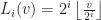


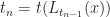


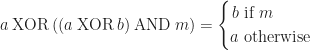


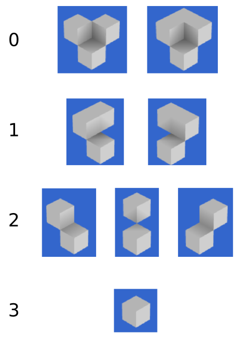

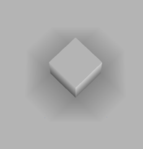


 , then it is also consistent with any subset of the views
  .
.
 , is visually consistent. So suppose by contradiction that it is not; then there exists some point
  . But by definition, there must be some visually consistent set
  containing
  . However, since
  is a strict subset, the number views in which
  is visible is a super set of the views containing it in


 regular grid, f, we project it down to a
  grid f’ according to the rule:


 , be a pair of shifted

 , we’d get:
 in red, and the shallower potential
  in blue. One can check that their zero-sublevel sets coincide:
 , observe what happens to their zero-crossings:


 , a class of simpler shapes
  on the space of all shapes, find some approximate shape
  such that
  is minimized:
 which is the best approximation of
  . This is probably the fastest method I’ve seen for simplifying an isosurface, but the speed comes at the cost of greater implementation complexity. But, if you are planning on doing mesh simplification, and you feel confident in your coding skills, then there is no practical reason not to use this technique.
 by sampling it onto a cubical grid at some fixed resolution. To get intermediate values, we’ll just interpolate between grid points using the standard
  generalization of Minecraft-style voxel surfaces. Our goal in this article is to figure out how to extract a mesh of the implicit surface (or zero-crossings of
  different possibilities, each of which is determined by the sign of the function at the 8 vertices of the cube:
 cases, a number which can be further reduced to just 3 special cases by symmetry considerations. This is enough that you can work them out by hand.


 volume plot of
![[ - \frac{\pi}{2}, + \frac{\pi}{2} ]^3](https://s0.wp.com/latex.php?latex=%5B+-+%5Cfrac%7B%5Cpi%7D%7B2%7D%2C+%2B+%5Cfrac%7B%5Cpi%7D%7B2%7D+%5D%5E3&bg=ffffff&fg=1a1a1a&s=0&c=20201002) . Here are the timings I got, measured in milliseconds
. Here are the timings I got, measured in milliseconds

 , it determines a set which we call the regularized 0-sublevel,
 to denote the
  is the closure (of the preimage of (the open interval
  ) ). Our definition of
  is a little bit different than the standard (but unfortunately slightly broken) definition which you see quite frequently:
![Z_0(f) \stackrel{def}{=} f^{-1}( [-\infty, 0] ) = \{ (x,y,z) \in \mathbb{R}^3 : f(x,y,z) \leq 0 \}](https://s0.wp.com/latex.php?latex=Z_0%28f%29+%5Cstackrel%7Bdef%7D%7B%3D%7D+f%5E%7B-1%7D%28+%5B-%5Cinfty%2C+0%5D+%29+%3D+%5C%7B+%28x%2Cy%2Cz%29+%5Cin+%5Cmathbb%7BR%7D%5E3+%3A+f%28x%2Cy%2Cz%29+%5Cleq+0+%5C%7D&bg=ffffff&fg=1a1a1a&s=0&c=20201002)
 . This has a pair of roots at
  , and looks like this:
 and
and ![[-1, 1]](https://s0.wp.com/latex.php?latex=%5B-1%2C+1%5D&bg=ffffff&fg=1a1a1a&s=0&c=20201002) . Where things break down however is near the edge cases. If for example we took the function
. Where things break down however is near the edge cases. If for example we took the function  :
:
 is not necessarily a

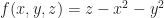


![\varphi : [0,1] \to \mathbb{R}^3](https://s0.wp.com/latex.php?latex=%5Cvarphi+%3A+%5B0%2C1%5D+%5Cto+%5Cmathbb%7BR%7D%5E3&bg=ffffff&fg=1a1a1a&s=0&c=20201002) , and then try to solve for the place where f composed with
, and then try to solve for the place where f composed with  crosses 0:
 .
.


 operations to perform a monotone subdivision, where
  is the number of vertices.
 algorithm out at the end of the day (where this


 .
. measures the algorithm dependent overhead which is determined by the complexity of the surface and the type of mesh generation. Since it is mesh generation that we want to study, ideally we’d like to keep
 .
. increases, the number of chambers increases as well, along with the surface area. This gives us a pretty good way to control for the complexity of surfaces in an experiment. I implemented this idea in a
  ). Garbage collection costs are amortized by repeated runs (10 in this case). All experiments were performed on a 65x65x65 volume with
  .
.

 quads, while in the culled version we’d get only
  . This gives an improvement of a factor of about

 , where
  is the upper left corner and
  is the width / height of the quad. Given such a representation of a quad, we denote its underlying set by:
![Q_{x,y,w,h} = \{ (s,t) \in \mathbb{R}^2 : x \leq s \leq x + w \: \mathrm{ and } \: y \leq t \leq y+h \} = [x,x+w] \times [y,y+h]](https://s0.wp.com/latex.php?latex=Q_%7Bx%2Cy%2Cw%2Ch%7D+%3D+%5C%7B+%28s%2Ct%29+%5Cin+%5Cmathbb%7BR%7D%5E2+%3A+x+%5Cleq+s+%5Cleq+x+%2B+w+%5C%3A+%5Cmathrm%7B+and+%7D+%5C%3A+y+%5Cleq+t+%5Cleq+y%2Bh+%5C%7D+%3D+%5Bx%2Cx%2Bw%5D+%5Ctimes+%5By%2Cy%2Bh%5D+&bg=ffffff&fg=1a1a1a&s=0&c=20201002)
 . Now let’s define a
  define the relation:
 such that
  and and
  , we can simply compare them lexicographically. Again, this new ordering is in fact a total order, and this means that it has a unique least element. In greedy meshing, we are going to take this least element as our mesh, which we’ll call the greedy mesh. Here is an example of what one of these lexicographically minimal meshes looks like:

 times smaller than the culled mesh for spherical geometries (where
 convex and
  concave vertices on the perimeter,
  .
. region with a perimeter of
  edges requires at least
  quads to mesh.
 denote the number of convex/concave vertices on the perimeter respectively. Because each quad can cover at most 4 convex vertices, the number of quads,
  , in the mesh is always at least
  . By the winding number theorem, it is true that for simply connected regions
  , and so
  . Therefore any mesh of a simply connected region requires at least
  quads. To extend this to non-simply connected regions, we observe that any quad mesh can be cut into a simply connected one by slicing along some edges in the quad mesh connecting out to the boundary. Making this cut requires introducing at most two edges per each hole in the object, and so we could just as well treat this as a simply connected region having
  edges, and applying the previous result gives us the bound in the lemma.
 . In summary, we have the following progression:
 Greedy


 .
.