I was getting a bit tired of the old theme I was using (Manifest) and decided to try something different. One nice thing with this new version is that it has a sidebar which makes it a bit easier to navigate around the blog. I’m also going to be adding some links to other blogs and resources on the sidebar over time.
If anyone has some further suggestions or ideas, please leave a comment!
Last time, we talked about an interesting generalization of Conway’s Game of Life and walked through the details of how it was derived, and investigated some strategies for discretizing it. Today, let’s go even further and finally come to the subject discussed in the title: Conway’s Game of Life for curved surfaces!
Quick Review: SmoothLife
To understand how this works, let’s first review Rafler’s equations for SmoothLife. Recall that is the state field and that we have two effective fields which are computed from f:
And that the next state of f is computed via the update rule:
Where:
And we have 6 (or maybe 7, depending on how you count) parameters that determine the behavior of the automata:
: The fraction of living neighbors required for a cell to stay alive (typically ).
: The fraction of living neighbors required for a cell to be born (typically ).
: The transition smoothness from live to dead (arbitrary, but Rafler uses ).
: Transition smoothness from interval boundary (again, arbitrary but usually about ).
: The size of the effective neighborhood (this is a simulation dependent scale parameter, and should not effect the asymptotic behavior of the system).
Non-Euclidean Geometry
Looking at the above equations, the only place where geometry comes into the picture is in the computation of the M and N fields. So it seems reasonable that if we could define the neighborhoods in some more generic way, then we could obtain a generalization of the above equations. Indeed, a similar idea was proposed in Rafler’s original work to extend SmoothLife to spherical domains; but why should we stop there?
Geodesic Distance
The basic idea behind all of this is that we want to generalize the concept of a sphere to include curved surfaces. Recall the usual definition of a sphere is that it is the set of all points within some distance of a given point. To extend this concept to surfaces, we merely have to change our definition of distance somewhat. This proceeds in two steps.
First, think about how the distance between two points is defined. In ordinary Euclidean geometry, it is defined using the Pythagorean theorem. That is if we fix a Cartesian coordinate system the distance between a pair of points is just:
But this isn’t the only way we could define this distance. While the above formula is pretty easy to calculate, it by far not the only way such a distance could be defined. Another method is that we can formulate the path length variationally. That is we describe the distance between points p and q as a type of optimization problem; that is it is the arc length of the shortest path connecting the two points:
At a glance this second statement may seem a bit silly. After all, solving an infinite dimensional optimization problem is much harder than just subtracting and squaring a few numbers. There is also something about the defining Euclidean distance in terms of arclength that seems viciously circular — since the definition of arclength is basically an infinitesimal version of the above equation — but please try not to worry about that too much:
Computing arclength by subdivisions. Image (c) Wikipedia 2007. Author: Mike Peel
Instead, the main advantage of working in the variational formulation is that it becomes possible to define distances in spaces where the shortest path between two points is no longer a straight line, as is the case on the surface of the Earth for example:
The shortest distance between any two cities on Earth is a circle — not a straight line!
Of course to define the arclength for something like a curve along a sphere, we need a little extra information. Looking at the definition of arclength, the missing ingredient is that we need some way to measure the length of a tangent vector. The most common way to do this is to introduce what is known as a Riemannian metric, and the data it stores is precisely that! Given a smooth manifold , a Riemannian metric continuously assigns to every point a symmetricbilinear form on the tangent space of at p. To see how this works let us, suppose we were given some curve , then we can just define the arclength of f to be:
Armed with this new generalization arclength, it is now pretty clear how we should define the distance between points on a Riemannian manifold (that is any differentiable manifold equipped with a Riemannian metric). Namely, it is:
This is called the geodesic distance between p and q, after the concept of a geodesic which is a fancy name for `the shortest path between two points’. The fact that concatenation of paths is associative implies that geodesic distance satisfies the triangle inequality, and so it is technically a metric. The fact that our metric is allowed to vary from point to point allows us to handle much more flexible topologies and and surfaces. For example, parallel or offset curves on a Riemannian manifold may not be straight lines. This leads to violations of Euclid’s parallel postulate and so the study of Riemannian manifolds is sometimes called non-Euclidean geometry. (It also has a few famous applications in physics!)
Geodesic Balls
Now that we have a definition of distance that works for any surface (with a Riemannian metric), let’s apply it to Rafler’s equations. I claim that all we need to do is replace the spherical neighborhoods in SmoothLife with some suitably constructed geodesic neighborhoods. In particular, we can define these neighborhoods to be balls of some appropriate radius. Given a point p, we define the geodesic ball of radius h centered at p to be the set of all points within distance at most h of p:
Which naturally leads to defining the M and N fields as follows:
That these equations constitute a generalization of SmoothLife to curved surfaces should be pretty clear (since we barely changed anything at all!). One can recover the original SmoothLife equations by setting and taking a flat metric. However, there is a major departure in that the very same equations can now be used to describe the dynamics of life on curved surfaces as well!
Discrete Riemannian Manifolds
Generalizing SmoothLife to surfaces didn’t change the equations much, but conceptually there is now a whole lot more to unpack. To actually implement this stuff, we need to solve the following three problems:
First, we need to figure out what metric to use.
Then, we need some way to compute geodesic balls on a surface.
Finally, we have to discretize the fields on the surface in some way.
The last part follows along more or less the same sort of reasoning as we applied in the periodic/flat case, (though the details are a bit different). However, items 1 and 2 are new to SmoothLife on curved surfaces and requires some special explanation.
Metric Embeddings
Up to this point, we’ve been deliberately abstract in our dealings with metrics, and haven’t really said much about where they come from. In the most general setting, we can think of a metric as something which is intrinsic to a surface — ie it is part of the very data which describes it. However, in practical applications — especially those arising in computer graphics and engineering — metrics usually come from an embedding. Here’s how it works:
Given a pair of differential manifolds and a smooth map with a metric on , then induces a metric on by a pullback. That is, be the differential of , then there ia metric on for every point :
To make this very concrete, let us suppose that our surface is sitting inside 3D Euclidean space. That is we have some smooth map that takes our surface and sticks it into 3-space with the ordinary flat Euclidean metric. Then the geodesic distance is just the length of the shortest path in the surface:
In the case of a triangulated mesh, we can let the embedding map just be the ordinary piecewise linear embedding of each triangle into 3-space.
Geodesics on Triangulated Surfaces
Ok, so now that we have a Riemannian metric, the next thing we need to is figure out how to calculate the geodesic distance. As far as I am aware, the first comprehensive solution to this problem was given by Mitchell, Mount and Papadimitrou back in 1987:
The basic idea behind their algorithm is pretty straightforward, though the details get a little hairy. It basically amounts to a modified version of Dijkstra’s algorithm that computes the single source shortest path to every point along each edge in the mesh. The basic reason this works is that within the interior of each face the actual distance field (for any point source) is always piecewise quadratic. However, there is a catch: the distance along each edge in the mesh might not be quadratic. Instead you may have to subdivide each edge in order to get a correct description of the distance field. Even worse, in that paper Mitchell et al. show that the exact distance field for a mesh with vertices could have distinct monotone components per edge, which gives their algorithm a worst case running time of , (the extra log factor is due to the cost associated with maintaining an ordered list for visiting the edges.)
Quadratic time complexity is pretty bad — especially for large meshes — but it is really about the best you can hope for if you are trying to solve the problem properly. In fact, a distance field on a piecewise linear triangular surface can have up to distinct piecewise polynomial components, and so you need bits just to encode the field anyway. However, it has been observed that in practice the situation is usually not so bad and that it is often possible to solve the problem faster if you are willing to make do with an approximation. Over the years, many alternatives and approximations to geodesic distance have been proposed, each making various trade offs. Here is a quick sampling of a few I found interesting:
The first two papers are important in that they describe different ways to look at approximating geodesic distance. Polthier and Schmies give an alternative definition of geodesic distance which is easier to calculate, while Kimmel and Sethian describe a method that approximates the surface itself. Both methods run in time instead of — though one needs to be a bit careful here, since the in Kimmel and Sethian (aka number of voxels) could actually be exponentially larger than the (number of vertices) which is used in the other papers (in practice this is usually not much of a problem). The last paper is also important as it is one of the most cited in this area, and discusses a simple a modification of Mitchell et al.’s method which gives some ability to make a tradeoff between performance and accuracy. I also like this paper for its clarity, since the figures are much easier to follow than the original 1987 work.
One conclusion that can be drawn from all this is that computing geodesic distance is a hairy problem. Digging around it is easy to get lost in a black hole of different possibilities. Since this is not the main point of this post (and because I wrote most of this code while I was on an airplane without access to the internet), I decided to try just hacking something together and ended up going with the first thing that worked. My approach was to use a modification of the Bellman-Ford algorithm and compute the geodesic distance in two phases. First, I did an iteration of Dijkstra’s algorithm on the edges of the mesh to get an upper bound on the distance, using the Euclidean distance lower bound to trim out far away vertices. Then I iterated unfolding the faces to try to refine the distance field until it converged.
This approach may be novel, but only because it is s obviously terrible compared to other techniques that no one would ever bother to publish it. Nonetheless, in my experiments I found that it gave a passable approximation to the distance field, provided that the mesh had enough subdivisions. The downside though is that the Bellman-Ford algorithm and its variants are quite slow. If I ever have the time, I’d like to revisit this problem some day and try out some better techniques and see how they compare, but that will have to be the subject of another entry. For now, this approach will have to do.
The Finite Element Method
Supposing that we now have some reasonable approximation to geodesic distance (and thus the shape of a geodesic ball) on our mesh, we now need to come up with a way to represent an approximation of the state field on the mesh. Just like in the flat version of SmoothLife, we must use the Galerkin method to discretize the system, but this time there is a major difference. When we were on a flat/periodic domain, we had the possibility of representing the field by a sum of Dirichlet or sinc elements, which turned out to make it really easy to calculate the effective fields M and N using the Fourier transform. However on an arbitrary curved surface (or mesh) we usually don’t have any sort of translational symmetry and so such a representation is not always possible.
Instead, we will have to make do with a somewhat more general, but less efficient, set of basis functions. In engineering applications, one popular choice is to write the field as a sum of splines, (aka smooth compactly supported piecewise polynomial functions). In fact, this idea of using the Galerkin method with splines is so widely used that it even has its own special name: the Finite Element Method (FEM). FEM is basically the default choice for discretizing something when you don’t really know what else to do, since it works for pretty much any sort of topology or boundary condition. The tradeoff is that it can be a lot less efficient than other more specialized bases, and that implementing it is usually much more complicated.
Piecewise Linear Elements
As a first attempt at creating a finite element discretization for SmoothLife, I opted to go with piecewise linear or `tent’ functions for my basis functions:
Illustration of a piecewise linear approximation by tent functions. Image (c) Wikipedia 2012. Author: Krishnavedala
For a 2D triangulated mesh, the simplest piecewise linear basis functions are the Barycentric coordinates for each face. To explain how this works, let us first describe how we can use these functions to parameterize a single triangle. In a Barycentric coordinate system, a triangle is described as a subset of :
The three vertices of the triangle correspond to the coordinates respectively. Using this coordinate system it is really easy to define a linear scalar function on . Pick any 3 weights and define a map according to the rule:
This formula should be pretty familiar if you know a bit about computer graphics. This is the same way a triangle gets mapped into 3D! To get a map from the triangle to any vector space, you can just repeat this type of process for each component separately.
Ok, now that we have some idea of how an embedding works for a single triangle let’s figure out how it goes for a complete mesh. Again we start by describing the parameter space for the mesh. Let us suppose that our mesh is abstractly represented by a collection of vertices, and faces, where each face, is a 3-tuple of indices into (in other words, it is an index array). To each vertex we associate a scalar and for every face we add a constraint:
The solution set of all of these constraints cuts out a subset of which is the parameter space for our mesh. To define a piecewise linear scalar field on , we just need to pick different weights, one per each vertex. Then we write any piecewise linear scalar field, , analgous to the triangular case:
In other words, the basis or `shape’ functions in our discretization are just the Barycentric coordinates . To see what this looks like visually, here is another helpful picture from wikipedia:
The 2D linear finite element shape functions visualized for a planar triangulation. The field is plotted above while the topology of the mesh is visualized on the bottom. Image (c) Wikipedia 2007. Author Oleg Alexandrov
Integration on Meshes
Now that we know our basis functions, we need to say a bit about how we integrate them. To do this, let us suppose that we have a piecewise linear embedding of our mesh which is specified (again in the linear shape functions) by giving a collection of vectors . These vertex weights determine an embedding of our mesh in 3D space according to the rule
To integrate a scalar function over the embedded surface , we want to compute:
This seems a little scary, but we can simplify it a lot using the fact that is piecewise linear over the mesh and instead performing the integration face-by-face. Integrating by substitution, we get:
The way you should read that is that every term is 0 except for the components, which are set to respectively.
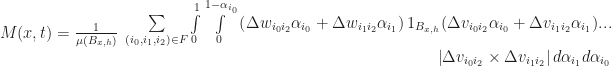
Computing the Effective Fields
Now let’s suppose that we have a state field and that we want to compute the effective fields $late M$ and as defined above. Then by definition:
The function is just the indicator function for the geodesic ball centered at x with radius h, and is computed using the geodesic distance field we described above. To actually evaluate the integral, let us suppose that is a weighted sum of linear shape functions:
Then we apply the expansion we just described in the previous section:
Where:
This integral is pretty horrible to compute analytically, but fortunately we don’t have to do that. Instead, we can approximate the true result by using a numerical quadrature rule. The way quadrature rules work is you just sample the integrand and take linear combinations of the results. For cleverly selected weights and sample points, this can even turn out to be exact — though working out exactly the right values is something of a black art. Fortunately, a detailed understanding of this process turns out to be quite unnecessary, since you can just look up the sample points and weights in a book and then plug in the numbers:
It should be obvious that the same trick works for computing , just by replacing with .
Matrix Formulation and Implementation
To compute the next state of , we can just sample the field at each vertex. To do this, let us define:
Then we can update according to the rule:
While this would work, it would also be very slow, since computing at each vertex requires doing quadratic work. Instead, it is better if we precalculate a bit to avoid doing so many redundant computations. To understand how this works, observe that our rule for computing the quantities is linear in the vector . This means that we can write it as a matrix:
Where are the vectors of coefficients and is the matrix which we precalculate whose entries using the formula:
That is, it is a sum over all the faces incident to vertex (which I wrote as to save space), with quadrature computed as described above. Since the outer radius for the cells are finite, ends up being pretty sparse and so it is relatively easy to process and store. Again, the same idea applies to the effective neighborhoods which we store in the matrix . Putting this together, we get the following algorithm:
Use geodesic distance to precompute matrices
Initialize state vector
For each time step:
Set
Set
Set
Demo
If you want to try playing around with this stuff yourself, I made a WebGL demo that should work in Chrome (though I haven’t tested it in Firefox). You can check it out here:
Be warned though! It is very slow due to the inefficient calculation of geodesic distances. Of course once it has finished assembling the matrices it runs pretty well in the browser. If you want to look at the code for the demo, you can try it out on github:
The project is written using node.js and has dependencies on two other libraries I made, namely trimesh.js and meshdata — both of which you can install via npm.
Conclusions
In conclusion, we’ve demonstrated the extended the domain of Rafler’s SmoothLife equations to curved surfaces. While our current implementation is somewhat crude, it does suffice to illustrate that the basic theoretical concepts are sound. In the future, it would be good to investigate alternative methods for computing geodesic distance. At the moment, this is the main bottleneck in the pipeline, and solving it would make further investigation of SmoothLife and related phenomena much easier.
It would also be interesting to attempt a more detailed analysis of the dynamics of SmoothLife. One interesting puzzle would be to try working out the stability of various solitons/gliders in the presence of curvature. It seems that they tend to destabilize and bifurcate near regions of high curvature. This is probably due to the fact that the soliton interacts with itself in these regions. For small curvatures, the trajectory of the solitons are deflected, causing gravitational like effects on their motion.
Conway’s Game of Life is one of the most popular and iconic cellular automata. It is so famous that googling it loads up a working simulation right in your browser! The rules for the Game of Life (GoL) can be stated in a few lines:
The world is an infinite rectangular array of cells, each of which can be in one of two states: alive or dead; and the neighborhood of each cell is a 3×3 grid centered on the cell.
The state of the world advances in discrete synchronous time steps according to the following two rules:
Cells which are alive remain alive if and only if they have between 2 and 3 neighbors; otherwise they die.
Cells which are dead become alive if they have exactly 3 neighbors; or else they stay dead.
Despite the superficial simplicity of these rules, the Game of Life can produce many unexpected and fascinating recurring patterns; like the glider soliton:
A 3×3 glider in Conway’s Game of Life. Black represents a live cell; white represents dead. (c) 2008, Wikipedia. Author: Dhatfield
The fact that the rules for the Game of Life are so short and clear makes it a great project for initiating novice programmers. Since Life was invented by John Conway in 1970, it has distracted many amateur and recreational mathematicians, leading to the discovery of many interesting patterns. For example, Paul Chapman showed that Life is Turing complete, and so it is in principle possible to translate any computer into a set of initial conditions. As an amusing example of this concept, here is an implementation of Conway’s Game of Life in the Game of Life created by Brice Due. Another cool pattern is the famous Gemini spaceship which is a complex self replicating system, and is perhaps the first true `organism’ to be discovered in life! If any of this sounds interesting to you, you can play around with the Game of Life (and some other cellular automata) and look at a large and interesting library of patterns collected in the community developed Golly software package.
SmoothLife
Now, if you’ve been programming for any reasonable length of time you’ve probably come across the Game of Life at least a couple of times before and so all the stuff above is nothing new. However, a few weeks ago I saw an incredibly awesome video on reddit which inspired me to write this post:
This video is of a certain generalization of Conway’s Game of Life to smooth spaces proposed by Stephan Rafler:
You can read this paper for yourself, but I’ll also summarize the key concepts here. Basically, there are two main ideas in Rafler’s generalization: First, the infinite grid of cells is replaced with an `effective grid’ that is obtained by averaging over a disk. Second, the transition functions are replaced by a series of differential equations derived from a smooth interpolation of the rules for the discrete Game of Life.
Effective Grids
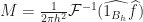
To explain how an `effective grid’ works, first consider what would happen if we replaced the infinite discrete grid in the game of life with a time-dependent continuous real scalar field, on the plane. Now here is the trick: Instead of thinking of this is an infinite grid of infinitesimal cells, we give the cells a small — but finite! — length. To do this, pick any small positive real number h which will act as the radius of a single cell (ie “the Planck length” for the simulation). Then we define the state of the `effective cell‘ at a point x as the average of the field over a radius h neighborhood around x, (which we call M(x,t) following the conventions in Rafler’s paper):
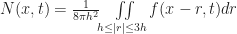
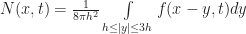
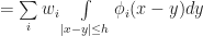
Now for each cell, we also want to compute the effective “number of cells” in its neighborhood. To do this, we use the same averaging process, only over a larger annulus centered at x. By analogy to the rules in the original GoL, a reasonable value for the outer radius is about 3h. Again, following Rafler’s conventions we call this quantity N(x,t):
To illustrate how these neighborhoods fit together, I made a small figure:
Now there are two things to notice about M and N:
They are invariant under continuous shifts.
They are invariant under rotations.
This means that if we define the state of our system in terms of these quantities, the resulting dynamics should also be invariant under rotations and shifts! (Note: These quantities are NOT invariant under scaling, since they are dependent on the choice of h.)
Smooth Transition Functions
Of course getting rid of the grid is only the first step towards a smooth version of Life. The second (and more difficult) part is that we also need to come up with a generalization of the rules for the game of life that works for continuous values. There are of course many ways to do this, and if you’ve taken a course on real analysis you may already have some idea on how to do this. However, for the sake of exposition, let’s try to follow along Rafler’s original derivation.
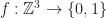
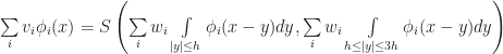
As a starting point, let’s first write the rules for the regular discrete Game of Life in a different way. By some abuse of notation, suppose that our field f was a discrete grid (ie ) and that N, M, give the state of each cell and the number of live cells in the 1-radius Moore neighborhood. Then we could describe the rules of Conway’s Game of Life using the equation:
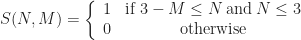
Where S represents the transition function of the Game of Life, and is defined to be:
Since S is a function of two variables, we can graph it by letting the x-axis be the number cells in the neighborhood and the y-axis be the state of the cell:
Plot of state transition for GoL. Y-axis is N, X-axis is M, red=alive, blue=dead.
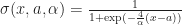
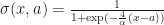
Now given such a representation, our task is to `smooth out’ S somehow. Again to make things consistent with Rafler, we first linearly rescale N, M so that they are in the range [0,1] (instead of from [0,9), [0,2) respectively). Our goal is to build up a smooth approximation to S using sigmoid functions to represent state transitions and thresholding (this is kind of like how artificial neural networks approximate discrete logical functions). Of course the term `sigmoid’ is not very precise since a sigmoid can be any function which is the integral of a bump. Therefore, to make things concrete (and again stay consistent with Rafler’s paper) we will use the logistic sigmoid:
It is a bit easier to understand what does if we plot it, taking :
Plot of the logistic sigmoid from x = -6 to 6. Image (c) Wikipedia 2008. Author Geoff Richards.
Intuitively, smoothly goes to 0 if x is less than a, and goes to 1 if x is greater than a. The parameter determines how quickly the sigmoid `steps’ from 0 to 1, while the parameter a shifts the sigmoid. Using a sigmoid, we can represent 0/1, alive/dead state of a cell in the effective field by thresholding:
The idea is that we think of effective field values greater than 0.5 as a live, and those less than 0.5 as dead. We can also adapt this idea to smoothly switch between any two different values depending on whether a cell is alive or dead:
The idea is that selects between a and b depending on whether the cell is dead or alive respectively. The other thing we will need is a way to smoothly threshold an interval. Fortunately, we can also do this using . For example, we could define:
Plot of for n=0 to 1
Putting it all together, let’s now make a state transition function which selects the corresponding interval based on whether the state of the cell is currently alive or dead:
Where are a pair of intervals which are selected based on user specified parameters. Based on the game of life, a reasonable set of choices should be , which if plotted gives a chart that looks something like this:
This is the transition function for SmoothLife as defined by Rafler. The squishing of this plot relative to the original plot is just a side effect of rescaling the axes to the unit interval, but even so the similarity is unmistakable. The only thing left is to pick the value of . In the original paper on SmoothLife, Rafler allows for two different values of ; for their appearance in respectively. Along with the bounds for the the life/death intervals , there are 6 total parameters to choose from in building a cellular automaton for SmoothLife.
Timestepping
Now, there is still one nagging detail. I have not yet told you how the time works in this new version of life. In Rafler’s paper he gives a couple of possibilities. One simple option is to just do discrete time stepping, for example:
However, this has the disadvantage that the time stepping is now discretized, and so it violates the spirit of SmoothLife somewhat. Another possibility (advocated in Rafler’s paper) is to rewrite this as a differential equation, giving the following smooth update rule:
I found this scheme to give poor results since it tends to diverge whenever the state of a cell is relatively stable (leading to field values outside the range [0,1]). (UPDATE: I just got an email from Stephan Rafler, apparently the equation I wrote earlier was wrong. Also, he recommends that the field values be clamped to [0,1] to keep them from going out of bounds.) A slightly better method which I extracted from the source code of SmoothLife is the following technique that pushes the state of the effective field towards S exponentially:
It is also possible to replace f(x,t) with M(x,t) on the right hand side of the above equations and get similar results. It is claimed that each of these rules can produce interesting patterns, though personally I’ve only observed the first and last choices actually working…
Discretizing SmoothLife
Now that we have the rules for SmoothLife, we need to figure out how to actually implement it, and to do this we need to discretize the field f somehow. One common way to do this is to apply the Galerkin method. The general idea is that for a fixed t, we write f as a weighted sum of simpler basis functions (which I will deliberately leave unspecified for now):
The undetermined weights are the degrees of freedom we use to represent . For example, we could represent f as a polynomial series expansion, in which case and the weights would just be the coefficients, . But there is no reason to stop at polynomials, we could approximate f by whatever functions we find convenient (and later on we’ll discuss a few reasonable choices.) What does this buy us? Well if we use a finite number of basis elements, , then we can represent our field f as a finite collection of numbers ! Cool! So, how do we use this in our simulation?
Well given that at time t, and supposing that at time t+1 we have , all we need to do is solve for the coefficients . This could be done (hypothetically) by just plugging in f(x,t), f(x,t+1) into both sides of Rafler’s SmoothLife update equation:
To compute M we just plug in f(x,t):
And a similar formula holds for N as well. Therefore, we have the equation:
Unfortunately, it is usually not the case that there is an exact solution to this equation. The underlying reason the above idea may fail is that it might not be possible to represent our solution in the basis functions exactly. So we have to modify the equation somewhat. Instead of trying to get a perfect solution (which is generally impossible for arbitrary nonlinear PDEs or crazy boundary conditions), we’ll settle for approximating the solution as best as possible. The way we do this that we seek to find a choice of which minimizes an error in some suitable metric. For example, we could try to solve the following the following optimization problem instead:
Minimize
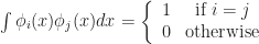
This type of system is sometimes called the weak formulation of the boundary value problem, and by standard linear algebra arguments finding the solution amounts to doing a subspace projection. In general this could be pretty annoying, but if we suppose that each of our were orthonormal — that is,
Then we know that,
and so all we have to do to compute the next state is integrate S(N,M) against each . A similar derivation applies for the smooth time stepping rules as well (modulo a small technical condition of that they must be differentiable).
Boundary Conditions
Ok, so we know (at least theoretically) what must be done to discretize the system. But how can we possibly hope to represent an infinite space using a finite number of basis functions? One simple solution is that we can make the space finite again by adding a periodicity condition. That is, let us require that for all x,y:
This means that we can parameterize the state of the infinite grid by just describing what happens within the region . This square is compact and so we have at least some hope of being able to approximate a periodic f by some finite number of functions covering this square.
Sinc Interpolation
Finally, we come to the point where we must pick a basis in order to go any further. There is some level at which the particular choice of representative functions is arbitrary and so one could reasonably justify almost any decision. For example, I could use B-splines, polynomials, sine waves, fractals or whatever I felt like (at least as long as I can integrate it to compute N and M). What I am going to describe here is by no means the only way to proceed. For example, in his paper Rafler uses a very simple bilinear expansion in terms of quadrilateral elements to get a decent discretization. (And if you want the details scroll up and read his write up).
However, because our system is periodic and translationally invariant (although not linear) there is one basis which has at least a somewhat more special status, and that is the Dirichlet or aliased sinc basis. Let R be the resolution of a uniform grid, and define:
Then we index our basis functions by a pair of indices with:
.
It may seem surprising at first, but these basis functions are actually orthogonal. If you’ve never seen something like this before, please don’t be alarmed! That definition (which seemed to come out of left field) is really a manifestation of the famous (and often misunderstood) Nyquist sampling theorem. It basically says that if we write any periodic, band limited function as a sum of sincs:
Then the weights are just the values of the function at the grid points:
This means that for any suitably smooth f, we can project it to our basis by just sampling it:
This makes our code way simpler, since we can avoid doing some messy numerical integration to get the weights. Assuming that S(N,M) is smooth enough (which in practice it is), then all we have to do to perform a discrete update is figure out how to compute M(x,y), N(x,y) for any given sinc expansion of f. In other words, we want to compute:
If you know a bit of Fourier analysis, you should know what comes next. Just take a Fourier transform and apply the convolution theorem to both sides, giving:
Which we can actually solve exactly, since the Nyquist theorem implies that is a finite sum. Therefore:
And by a bit of calculus, the Fourier transform of can be computed in closed form using Bessel functions. This means that:
A similar formula for N(x,y,t) can be obtained by writing:
Putting it all together, let be the new weights for f at time t+1. Then to do a discrete time step we just set:
I’ll leave it as an exercise to work out the update rules for the continuous time steps.
Implementation Details
Great, so we have some formulas for computing the next time step, but if we do it in a dumb way it is going to be pretty slow. The reason is that each of the above steps requires summing up all the coefficients of f to calculate M and N at each point, which is going to take linear work with respect to the number of terms in our summation. Spread out over all the points in the grid, this makes the total update . However, because the above sums are all Fourier series we can speed this up a lot using a fast Fourier transform. Basically we precalculate the weights by evaluating the Bessel function at each frequency, then at each time step we Fourier transform f, multiply by the weights, inverse transform and repeat. Here is what it looks like:
Initialize f
Precalculate
For t=1 to n
Use FFT to compute
Set
Set
Set
And that’s it!
Demo
If you want to try out SmoothLife yourself in your browser, I made a few jsFiddles which illustrate the basic principle. Here is a Fourier based implementation that follows the discussion in this article pretty closely:
You can run either of them in your browser and try changing the parameters.
Next Time…
The stuff in this article is basically background material, and most of it can be found in Rafler’s paper or is already more-or-less documented in the source code for the SmoothLife project on SourceForge. However, in the sequel I plan to go a bit farther than the basic rules for SmoothLife and tell you how to make a version of SmoothLife for curved surfaces!
 is the state field and that we have two effective fields which are computed from f:


![[b_1, b_2]](https://s0.wp.com/latex.php?latex=%5Bb_1%2C+b_2%5D&bg=ffffff&fg=1a1a1a&s=0&c=20201002) : The fraction of living neighbors required for a cell to stay alive (typically
: The fraction of living neighbors required for a cell to stay alive (typically ![[\frac{2}{8}, \frac{3}{8}]](https://s0.wp.com/latex.php?latex=%5B%5Cfrac%7B2%7D%7B8%7D%2C+%5Cfrac%7B3%7D%7B8%7D%5D&bg=ffffff&fg=1a1a1a&s=0&c=20201002) ).
).![[d_1, d_2]](https://s0.wp.com/latex.php?latex=%5Bd_1%2C+d_2%5D&bg=ffffff&fg=1a1a1a&s=0&c=20201002) : The fraction of living neighbors required for a cell to be born (typically
: The fraction of living neighbors required for a cell to be born (typically  ).
). : The transition smoothness from live to dead (arbitrary, but Rafler uses
  ).
). : Transition smoothness from interval boundary (again, arbitrary but usually about
  ).
). : The size of the effective neighborhood (this is a simulation dependent scale parameter, and should not effect the asymptotic behavior of the system).
 is just:
![d(p,q) = \min \limits_{f : [0,1] \to \mathbb{R}^2\\f(0)=p, f(1)=q} \int \limits_0^1 |\partial_t f(t)| dt](https://s0.wp.com/latex.php?latex=d%28p%2Cq%29+%3D+%5Cmin+%5Climits_%7Bf+%3A+%5B0%2C1%5D+%5Cto+%5Cmathbb%7BR%7D%5E2%5C%5Cf%280%29%3Dp%2C+f%281%29%3Dq%7D+%5Cint+%5Climits_0%5E1+%7C%5Cpartial_t+f%28t%29%7C+dt&bg=ffffff&fg=1a1a1a&s=0&c=20201002)


 , a Riemannian metric continuously assigns to every point
  a
a  on the
 ![f : [0,1] \to M](https://s0.wp.com/latex.php?latex=f+%3A+%5B0%2C1%5D+%5Cto+M&bg=ffffff&fg=1a1a1a&s=0&c=20201002) , then we can just define the arclength of f to be:
, then we can just define the arclength of f to be: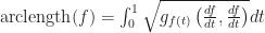
![d(p,q)=\min \limits_{\begin{array}{c} f : [0,1] \to M, \\ f(0) = p, f(1)=q\end{array}} \int_0^1 \sqrt{g_{f(t)} \left( \frac{d f}{dt}, \frac{d f}{dt} \right)} dt](https://s0.wp.com/latex.php?latex=d%28p%2Cq%29%3D%5Cmin+%5Climits_%7B%5Cbegin%7Barray%7D%7Bc%7D+f+%3A+%5B0%2C1%5D+%5Cto+M%2C+%5C%5C+f%280%29+%3D+p%2C+f%281%29%3Dq%5Cend%7Barray%7D%7D+%5Cint_0%5E1+%5Csqrt%7Bg_%7Bf%28t%29%7D+%5Cleft%28+%5Cfrac%7Bd+f%7D%7Bdt%7D%2C+%5Cfrac%7Bd+f%7D%7Bdt%7D+%5Cright%29%7D+dt&bg=ffffff&fg=1a1a1a&s=0&c=20201002)


 and taking a flat metric. However, there is a major departure in that the very same equations can now be used to describe the dynamics of life on curved surfaces as well!
 and a smooth map
  with a metric
  on
on  , then
  induces a metric on
  by a
by a  be the differential of
  on
on  :
:
 that takes our surface and sticks it into 3-space with the ordinary flat Euclidean metric. Then the geodesic distance is just the length of the shortest path in the surface:
![d(p,q) = \min_{f : [0,1] \to \Omega \\ f(0)=p, f(1)=q} \int_0^1 | \frac{d h(f(t))}{dt} | dt](https://s0.wp.com/latex.php?latex=d%28p%2Cq%29+%3D+%5Cmin_%7Bf+%3A+%5B0%2C1%5D+%5Cto+%5COmega+%5C%5C+f%280%29%3Dp%2C+f%281%29%3Dq%7D+%5Cint_0%5E1+%7C+%5Cfrac%7Bd+h%28f%28t%29%29%7D%7Bdt%7D+%7C+dt&bg=ffffff&fg=1a1a1a&s=0&c=20201002)
 vertices could have
  , (the extra log factor is due to the cost associated with maintaining an ordered list for visiting the edges.)
 distinct piecewise polynomial components, and so you need
  time instead of
  in Kimmel and Sethian (aka number of voxels) could actually be exponentially larger than the
  piecewise linear or `tent’ functions for my basis functions:
 :
:
 respectively. Using this coordinate system it is really easy to define a linear scalar function on
  . Pick any 3 weights
  and define a map
  according to the rule:
 and
and  faces,
  where each face,
  is a 3-tuple of indices into
 ![\alpha_0, \alpha_1, ... \alpha_{n-1} \in [0,1]](https://s0.wp.com/latex.php?latex=%5Calpha_0%2C+%5Calpha_1%2C+...+%5Calpha_%7Bn-1%7D+%5Cin+%5B0%2C1%5D&bg=ffffff&fg=1a1a1a&s=0&c=20201002) and for every face we add a constraint:
and for every face we add a constraint:
 which is the parameter space for our mesh. To define a piecewise linear scalar field on
  , we just need to pick
  , analgous to the triangular case:
 . To see what this looks like visually, here is another helpful picture from wikipedia:
 . These vertex weights determine an embedding of our mesh in 3D space according to the rule
 , we want to compute:
 is piecewise linear over the mesh and instead performing the integration face-by-face.
 is that every term is 0 except for the
  components, which are set to
  respectively.
 is just the indicator function for the geodesic ball centered at x with radius h, and is computed using the geodesic distance field we described above. To actually evaluate the integral, let us suppose that
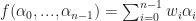

 .
.

 at each vertex requires doing quadratic work. Instead, it is better if we precalculate a bit to avoid doing so many redundant computations. To understand how this works, observe that our rule for computing the quantities
  is linear in the vector
  . This means that we can write it as a matrix:
 are the vectors of coefficients and
  is the matrix which we precalculate whose entries using the formula:
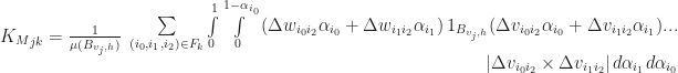
 (which I wrote as
  to save space), with quadrature computed as described above. Since the outer radius for the cells are finite,
  . Putting this together, we get the following algorithm:


 on the plane. Now here is the trick: Instead of thinking of this is an infinite grid of infinitesimal cells, we give the cells a small — but finite! — length. To do this, pick any small positive real number h which will act as the radius of a single cell (ie “the Planck length” for the simulation). Then we define the state of the `effective cell‘ at a point x as the average of the field over a radius h neighborhood around x, (which we call M(x,t) following the conventions in Rafler’s paper):
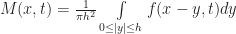

 ) and that N, M, give the state of each cell and the number of live cells in the 1-radius
 does if we plot it, taking
  :
:
 from x = -6 to 6. Image (c) Wikipedia 2008. Author Geoff Richards.
 determines how quickly the sigmoid `steps’ from 0 to 1, while the parameter a shifts the sigmoid. Using a sigmoid, we can represent 0/1, alive/dead state of a cell in the effective field by thresholding:

 selects between a and b depending on whether the cell is dead or alive respectively. The other thing we will need is a way to smoothly threshold an interval. Fortunately, we can also do this using
  . For example, we could define:

 for n=0 to 1
![[b_1, d_1], [b_2, d_2]](https://s0.wp.com/latex.php?latex=%5Bb_1%2C+d_1%5D%2C+%5Bb_2%2C+d_2%5D&bg=ffffff&fg=1a1a1a&s=0&c=20201002) are a pair of intervals which are selected based on user specified parameters. Based on the game of life, a reasonable set of choices should be
are a pair of intervals which are selected based on user specified parameters. Based on the game of life, a reasonable set of choices should be 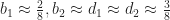 , which if plotted gives a chart that looks something like this:
 for their appearance in
  respectively. Along with the bounds for the the life/death intervals
  , there are 6 total parameters to choose from in building a cellular automaton for SmoothLife.
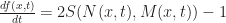

 (which I will deliberately leave unspecified for now):
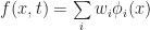
 . For example, we could represent f as a polynomial series expansion, in which case
  and the weights would just be the coefficients,
  . But there is no reason to stop at polynomials, we could approximate f by whatever functions we find convenient (and later on we’ll discuss a few reasonable choices.) What does this buy us? Well if we use a finite number of basis elements,
 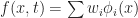 at time t, and supposing that at time t+1 we have
 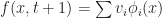 , all we need to do is solve for the coefficients
  . This could be done (hypothetically) by just plugging in f(x,t), f(x,t+1) into both sides of Rafler’s SmoothLife update equation:
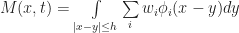
 error in some suitable metric. For example, we could try to solve the following the following optimization problem instead:


 . This square is compact and so we have at least some hope of being able to approximate a periodic f by some finite number of functions covering this square.
 with:
with: .
.
 are just the values of the function at the grid points:


 is a finite sum. Therefore:
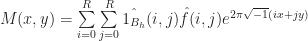
 can be computed in closed form using Bessel functions. This means that:
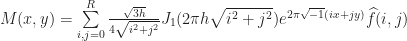

 be the new weights for f at time t+1. Then to do a discrete time step we just set: