Collision detection (part 3): Benchmarks

Previously in this series we covered the basics of collision detection and discussed some different approaches to finding intersections in sets of boxes:

Today, we’ll see how well this theory squares with reality and put as many algorithms as we can find to the test.  For those who want to follow along with some code, here is a link to the accompanying GitHub repo for this article:

The Great JavaScript Box Intersection Benchmark

Finding modules

To get a survey of the different ways people solve this problem in practice, I searched GitHub, Google and npm, and also took several polls via IRC and twitter.  I hope that I managed to cover most of the popular libraries, but if there is anything here that I missed, please leave a comment and let me know.

While it is not an objective measurement, I have also tried to document my subjective experiences working each library in this benchmark.  In terms of effort, some libraries took far less time to install and configure than others.  I also took notes on libraries which I considered, but rejected for various reasons.  These generally could be lumped into 3 categories:

  1. Broken: The library did not report correct results.
  2. Too much work: Setting up the library took too long.  I was not as rigorous with enforcing a tight bound here, as I tended to give more generous effort to libraries which were popular or well documented.  Libraries with 0 stars and no README I generally skipped over.
  3. Irrelevant: While the library may have at first looked like it was relevant, closer inspection revealed that it did not actually solve the problem of box intersection.  This usually happened because the library had a suspicious name, or because it was some framework whose domain appeared to include this problem.

A word on JavaScript

For the purpose of this benchmark, I limited myself to consider only JavaScript libraries. One major benefit of JavaScript is that it is easier to install and configure JavaScript libraries, which greatly simplifies the task of comparing a large number of systems.  Also, due to the ubiquity of JavaScript, it is easy for anyone to replicate these results or rerun these benchmarks on their own machine.  The disadvantage though is that there are not as many mature geometry processing libraries for JavaScript as there are for older languages like C++ or Java.  Still, JS is popular enough that I had no trouble finding plenty of things to test although the quality of these modules turned out to be wildly varying.

Implementations surveyed

Brute force

As a control I implemented a simple brute force O(n^2) algorithm in the obvious way.  While it is not efficient for large problem sizes, it performs pretty well up to few hundred points.

Bounding volume hierarchy modules

I found many modules implementing bounding volume hierarchies, usually in the form of R-trees.  Here is a short summary of the ones which I tested:

  • rbush:  This is one of the fastest libraries for box intersection detection.  It also has a very simple API, though it did take a bit of time tuning the branching factor to get best performance on my machine.  I highly recommend checking this one out!
  • rtree: An older rtree module, which appears to have largely been replaced by rbush.  It has more features, is more complicated, and runs a bit slower.  Still pretty easy to use though.
  • jsts-strtree:  The jsts library is a JavaScript port of the Java Topology Suite.  Many of the core implementations are solid, but the interfaces are not efficient.  For example, they use the visitor pattern instead of just passing a closure to enumerate objects which requires lots of extra boilerplate.  Overall found it clumsy to use, but reasonably performant.
  • lazykdtree: I included this library because it was relatively easy to set up, even though it ended up being very slow.  Also notable for working in any dimension.

Quad trees

Because of their popularity, I decided to make a special section for quad trees.  By a survey of modules on npm/GitHub, I would estimate that quad trees are one of the most commonly implemented data structures in JavaScript. However it is not clear to me how much of this effort is serious.  After much searching, I was only able to find a small handful of libraries that correctly implemented quad trees based rectangle stabbing:

  • simple-quadtree: Simple interface, but sluggish performance.
  • jsts-quadtree:  Similar problems as jsts-strtree.  Unlike strtree, also requires you to filter out the boxes by further pruning them against your query window.  I do not know why it does this, but at least the behavior is well documented.

Beyond this, there many other libraries which I investigated and rejected for various reasons.  Here is a (non-exhaustive) list of some libraries that didn’t make the cut:

  • Google’s Closure Library: This library implements something called “quadtree”, but it doesn’t support any queries other than set membership.  I am still not sure what the point of this data structure is.
  • quadtree2: Only supports ball queries, not boxes
  • Mike Chamber’s QuadTree: Returns incorrect results
  • quadtree-javascript: Returns incorrect results
  • node-trees: Returns incorrect results
  • giant-quadtree: Returns incorrect results
  • generic-quadtree:  Only implements point-in-rectangle queries, not rectangle-rectangle (stabbing) queries.
  • quadtree: I’m don’t know what this module does, but it is definitely not a quad tree.

Physics engines

Unfortunately, many of the most mature and robust collision detection codes for JavaScript are not available as independent modules.  Instead, they come bundled as part of some larger “physics framework” which implements multiple algorithms and a number of other features (like a scene graph, constraint solver, integrator, etc.).  This makes it difficult to extract just the collision detection component and apply it to other problems.  Still, in the interest of being comprehensive, I was able to get a couple of these engines working within the benchmark:

  • p2.js:  A popular 2D physics engine written from the ground up in JavaScript.  Supports brute force, sweep and prune and grid based collision detection.  If you are looking for a good 2D physics engine, check this one out!
  • Box2D: Probably the de-facto 2D physics engine, has been extremely influential in realtime physics and game development.  Unfortunately, the quality of the JS translations are much lower than the original C version.  Supports sweep-and-prune and brute force for broad phase collision detection.
  • oimo.js:  This 3D physics engine is very popular in the THREE.js community.  It implements brute force, sweep and prune and bounding volume hierarchies for collision detection.  Its API is also very large and makes heavy use of object-oriented programming, which comes with some performance tradeoffs. However oimo does deserve credit for being one of the few libraries to tackle 3D collision detection in JavaScript.

I also considered the following physics engines, but ended up rejecting them for various reasons:

  • cannon.js: To its credit, cannon.js has a very clear API and well documented code.  It is also by the same author as p2.js, so it is probably good.  However, it uses spheres for broad phase collision detection, not boxes, and so it is not eligible for this test.
  • GoblinPhysics:  Still at very early stages.  Right now only supports brute force collision detection, but it seems to be progressing quickly.  Probably good to keep an eye on this one.
  • PhysicsJS:  I found this framework incredibly difficult to deal with.  I wasted 2 days trying to get it to work before eventually giving up.  The scant API documentation was inconsistent and incomplete.  Also, it did not want to play nice in node.js or with any other library in the browser, hooking event handlers into all nooks and crannies of the DOM, effectively making it impossible to run as a standalone program for benchmarking purposes.  Working with PhysicsJS made me upset.
  • Matter.js:  After the fight with PhysicsJS, I didn’t have much patience for dealing with large broken libraries.  Matter.js seems to have many of the same problems, again trying to patch a bunch of weird stuff onto the window/DOM on load, though at least the documentation is better.  I spent about an hour with it before giving up.
  • ammo.js/physijs: This is an emscripten generated port of the popular bullet library, however due to the translation process the API is quite mangled.  I couldn’t figure out how to access any of the collision detection methods or make it work in node, so I decided to pass on it.

Range-trees

Finally, I tried to find an implementation of segment tree based intersection for JavaScript, but searching turned up nothing.  As far as I know, the only widely used implementation of these techniques is contained in CGAL, which comes with some licensing restrictions and also only works in C++.  As a result, I decided to implement of Edelsbrunner & Zomorodian’s algorithm for streaming segment trees myself.  You can find the implementation here:

box-intersect: Fast and robust d-dimensional box intersection

The code is available under a liberal MIT license and easily installable via npm.  It should work in any modern CommonJS environment including browserify, iojs and node.js.

Testing procedure

In each of these experiments, a set of n boxes was generated, and then sent to each library to compute a checksum of the set of pairs of intersections.  Because different libraries expect their inputs in different formats, as a preprocessing step the boxes are converted into whatever data type is expected by the library.  This conversion step is not counted towards the total running time.  Note that the preparation phase does not include any time required to build associated data structures like search trees or grids; these timings are counted toward the total run time.

Because algorithms for collision detection are output sensitive, care was taken to ensure that the total number of intersections in each distribution is at most O(n), in order to avoid measuring the reporting time for each method.

A limitation of this protocol is that it favors batched algorithms (as would be typically required in CAD applications), and so it may unfairly penalize iterative algorithms like those used in many physics engines.  To assess the performance of algorithms in the context of dynamic boxes more work would be needed.

Results

Here is a summary of the results from this benchmark.  For a more in depth analysis of the data, please see the associated GitHub repo.  All figures in this work were made with plot.ly, click on any of the images to get an interactive version.

Uniform distribution

I began this study by testing each algorithm against the uniform distribution.  To ensure that the number of intersections is at most O(n), I borrowed a trick from Edelsbrunner and Zomorodian; and scaled the side length of each box to be O(n^{\frac{1}{d}-1}) while constraining the boxes to remain within the unit hypercube, [0,1]^d.  A typical sample from this distribution looks like this,

Uniformly distributed boxes with side lengths
Uniformly distributed boxes

To save time, I split the trials into phases ordered by number of boxes; algorithms which performed took too long on smaller instances were not tested on larger problem sizes.  One of the first and most shocking results was a test instance I ran with just 500 boxes:

Click to inspect

Here two libraries stand out for their incredibly bad performance: Box2D and lazykdtree. I am not sure why this situation is so bad, since I believe the C version of Box2D does not have these problems (though I need to verify this).  Scaling out to 1500 boxes without these two libraries gives the following results:

Click to inspect

The next two worst performing libraries were simple-quadtree and rtree.  simple-quadtree appears to have worse than quadratic growth, suggesting fundamental algorithmic flaws.  rtree’s growth is closer to O(n \:\mathrm{polylog}(n)), but due to the constants involved is still far too slow.  As it took too long and there were 2 other representatives of the r-tree data structure in the benchmark, I decided to drop it from larger tests.  Moving on to 10k boxes,

Click to inspect

At this point, the performance of brute force begins to grow too large, and so it was omitted from the large brute force tests.

Because p2’s sweep method uses an insertion sort, it takes O(n^2) time with a cold start.  This causes it to perform close to brute force in almost all cases which were considered.  I suspect that the results would be better if p2 was used from a warm start or in a dynamic environment.

Both of jsts’ data structures continue to trend at about O(n \log(n)) growth, however because the constants involved are so large they were also dropped from the large problem size.

10000 boxes appears to be the cut off for real time simulation (or 60fps) at least on my machine.  Beyond, this point, even the fastest collision detection algorithm (in this case box-intersect) takes at least 16ms.  It is unlikely that any purely JavaScript collision detection library would be able to handle significantly more boxes than this, barring substantial improvements in either CPU hardware or VM technology.

One surprise is that within this regime, box-intersect is consistently 25-50% faster than p2-grid, even though one would expect the O(n) complexity of the grid algorithm to beat the O(n \log^2(n)) time of box-intersect.  An explanation for this phenomenon would be that box-intersect enjoys better cache locality (scaling linearly with block size), while hashing causes O(1) indirect main memory accesses for each box.  If the size of a cache line is B, then the cross over point should occur when n \approx \Theta(2^{\sqrt{B}}) in 2D.  This is illustrated in the following chart which carries out the experiment to 250k boxes,

Click to inspect

As expected, somewhere between 10000 and 20000 boxes, p2-grid finally surpasses box-intersect.  This is expected as grids realize O(n) complexity for uniform distributions, which is ultimately faster than O(n \log^2(n)) for sufficiently large n.

The complexity of rbush on this distribution is more subtle.  For the bulk insertion method, rbush uses the “overlap minimizing tree” (OMT) heuristic of Lee and Lee,

T. Lee, S. Lee. (2003) “OMT: Overlap minimizing top-down bulk loading algorithm for R-Trees” CAiSE

The OMT heuristic partitions the space into an adaptive R \times R grid at each level of the tree along the quantiles.  In the case of a uniform distribution of boxes, this reduces to uniform grid giving a query time of O( R^2 \log_{R^2}(n) + k), which for finite R gives means that rbush will find all intersections in O(n \log(n) + k) time.  As a result, we can expect that once n \approx \Theta(2^B), rbush-bulk should eventually surpass box-intersect in performance (though this did not occur in my benchmarks).  This also suggests another way to interpret the OMT heuristic:  it is basically a hedged version of the uniform grid.  While not quite as fast in the uniform case, it is more adaptive to sparse data.

Sphere

Of course realistic data is hardly ever uniformly distributed.  In CAD applications, most boxes tend to be concentrated in a lower dimensional sub-manifold, typically on the boundary of some region.  As an example of this case, we consider boxes which are distributed over the surface of a sphere (again with the side lengths scaled to ensure that the expected number of collisions remains at most O(n)).

A collection of boxes distributed over the boundary of ball.

To streamline these benchmarks, I excluded some of the worst performing libraries from the comparison.  Starting with a small case, here are the results:

Click to inspect

Again, brute force and p2’s sweep reach similar O(n^2) performance.

More significantly, p2-grid did not perform as well as in the uniform case, running an order of magnitude slower.  This is as theory would predict, so no real surprises.  Continuing the trend out to 50k boxes gives the following results,

Click to inspect

Both p2-grid and jsts-quadtree diverge towards O(n^2), as grid based partitioning fails for sparse data.

Both rbush and jsts-strtree show similar growth rates, as they implement nearly identical algorithms, however the constant factors in rbush are much better.  The large gap in their performance can probably be explained by the fact that jsts uses Java style object oriented programming which does not translate to JavaScript well.

One way to understand the OMT heuristic in rbush, is that it is something like a grid, only hedged against sparse cases (like this circle).  In the case of a uniform distribution, it is not quite as fast as a grid, suffering a O(\log(n)) penalty, while adding robustness against sparse data.

Again box-intersect delivers consistent O(n \log^2(n) + k) performance, as predicted.

High aspect ratio

Finally, we come to the challenging case of high aspect ratio boxes.  Here we generate boxes which are uniformly distributed in x and and stretched along the y-axis by a factor of O(n):

A set of boxes with a high aspect ratio

High aspect ratio boxes absolutely destroy the performance of grids and quad trees, causing exponential divergence in complexity based on the aspect ratio.  Here are some results,

Click to inspect

Even for very small ngrids take almost a second to process all intersections for just 10000 boxes.  This number can be made arbitrarily high by choosing as extreme an aspect ratio as one likes.  Here I select an aspect ratio of O(n), forcing the asymptotic growth of both jsts-quadtree and p2-grid to be O(n^2).  If I had selected the aspect ratio as O(2^n) or O(\infty), then it would have been possible to increase their running times to some arbitrarily large value.  In this benchmark, rbush also grows though by a much slower O(n^\frac{3}{2}).  Continuing out to 100k boxes, eventually rbush also fails,

Click to inspect

In this case rbush-bulk takes more than 40x slower and rbush-bulk more than 70x. Unlike in the case of grids however, these numbers are only realized by scaling in the number of boxes and so they cannot be made arbitrarily large.  However, it does illustrate that for certain inputs rbush will fail catastrophically.  box-intersect again continues to grow very slowly.

3D

The only libraries which I found that implemented 3D box intersection detection were lazykdtree and oimo.js.  As it is very popular, I decided to test out oimo’s implementation on a few small problem sizes.  Results like the following are typical:

Click here to inspect

Conclusions

For large, uniform distributions of boxes, grids are still the best.  For everything else, use segment trees.

  • Brute force is a good idea up to maybe 500 boxes or so.
  • Grids succeed spectacularly for large, uniform distributions, but fail catastrophically for anything more structured.
  • Quad trees (at least when properly implemented) realize similar performance as grids.  While not as fast for uniform data, they are slightly hedged against boxes of wildly variable size.
  • RTrees with a tuned heuristic can give good performance in many practical cases, but due to theoretical limitations (see the previous post), they will always fail catastrophically in at least some cases, typically when dealing with boxes having a high aspect ratio.
  • Zomorodian & Edelsbrunner’s streaming segment tree algorithm gives robust worst case O(n \log^d(n) + k) performance no matter what type of input you throw at it.  It is even faster than grids for uniform distributions at small problem sizes(<10k) due to superior cache performance.

Overall, streaming segment trees are probably the safest option to select as they are fastest in almost every case.  The one exception is if you have a large number of uniformly sized boxes, in which case you might consider using a grid.

Collision detection (part 2): Box intersection

Last time, we discussed collision detection in general and surveyed some techniques for narrow phase collision detection.  In this article we will go into more detail on broad phase collision detection for closed axis-aligned boxes.  This was a big problem in the 1970’s and early 1980’s in VLSI design, which resulted in many efficient algorithms and data structures being developed around that period.  Here we survey some approaches to this problem and review a few theoretical results.

Boxes

A box is a cartesian product of intervals, so if we want to represent a d-dimensional box, it is enough to represent a tuple of d 1-dimensional intervals.  There are at least two ways to do this:

  • As a point with a length
  • As a pair of upper and lower bounds

For example, in 2D the first form is equivalent to representing a box as a corner point together with its width and height (e.g. left, top, width, height), while the second is equivalent to storing a pair of bounds (e.g. [x_{min}, x_{max}] \times [y_{min}, y_{max}]).

A 2D box is the cartesian product of two intervals.
A 2D box is the cartesian product of two 1D intervals.

To test if a pair of boxes intersect, it is enough to check that their projections onto each coordinate axes intersects. This reduces the d-dimensional problem of box intersection testing to the 1D problem of detecting interval overlap.  Again, there are multiple ways to do this depending on how the intervals are represented:

  • Given two intervals represented by their center point and radius, [x_0-r_0, x_0+r_0], [x_1-r_1, x_1+r_1],

[x_0-r_0, x_0+r_0] \cap [x_1-r_1, x_1+r_1] \neq \emptyset \Longleftrightarrow |x_0 - x_1| \leq r_0 + r_1

  • Given two intervals represented by upper and lower bounds, [l_0, h_0], [l_1, h_1],

[l_0, h_0] \cap [l_1, h_1] \neq \emptyset \Longleftrightarrow l_0 \leq h_1 \wedge l_1 \leq h_0

In the first predicate, we require two addition operations, one absolute value and one comparison, while the second form just uses two comparisons.  Which version you prefer depends on your application:

  1. In my experiments, I found that the first test was about 30-40% faster in Chrome 39 on my MacBook, (though this is probably compiler and architecture dependent so take it with a grain of salt).
  2. The second test is more robust as it does not require any arithmetic operations.  This means that it cannot fail due to overflow or rounding errors, making it more suitable for floating point inputs or applications where exact results are necessary.  It also works with unbounded (infinite) intervals, which is useful in many problems.

For applications like games where speed is of the utmost importance, one could make a case for using the first form.  However, in applications where it is more important to get correct results (and not crash!) robustness is a higher priority.  As a result, we will generally prefer to use the second form.

1D interval intersection

Before dealing with the general case of box intersections in d-dimensions, it is instructive to look at what happens in 1D.  In the 1D case, there is an efficient sweep line algorithm to report all intersections.  The general idea is to process the end points of each interval in order, keeping track of all the intervals which are currently active.  When we reach the start of a new interval, we report intersections with all currently active intervals and it to the active set, and when we reach the end of an interval we delete the interval from the active set:

Finding all intersections in a set of intervals in 1D

In JavaScript, it looks something like this:

function sweepIntervals(intervals) {
  var events = [], result = [], active = []
  intervals.forEach(function(interval, id) {
    events.push(
      { t: interval[0], id: id, create: 1 },
      { t: interval[1], id: id, create: 0 })
  })
  events.sort(function(a, b) {
    return a.t - b.t || b.create - a.create
  })
  events.forEach(function(ev) {
    if(ev.create) {
      active.forEach(function(id) {
        result.push([ev.id, id])
      })
      active.push(ev.id)
    } else
      active.splice(active.indexOf(ev.id), 1)
  })
  return result
}

If the number of intervals is n, then there are O(n) events total, and so sorting them all takes O(n \log(n)) time.  Processing event requires a scan through the active set, however for each iteration one intersecting pair is reported.  If the total number of collisions is k, then the amortized cost of looping over the events is O(n + k).  Therefore, the total running time of this algorithm is in O(n \log(n) + k).

Sweep and prune

Sweeping is probably the best solution for finding interval overlaps in 1D.  The challenge is to generalize this to higher dimensions somehow.  One approach is to just run the 1D interval sweep to filter out collisions along some axis, and then use a brute force test to filter these pairs down to an exact set,

The sweep and prune method for box intersection detection.

In JavaScript, here is an illustration of how it could be implemented in terms of the previous 1D sweep algorithm:

//Assume each box is represented by a list of d intervals
//Each interval is of the form [lo,hi]
function sweepAndPrune(boxes) {
  return sweepIntervals(boxes.map(function(box) {
    return box[0]
  }).filter(function(pair) {
    var A = boxes[pair[0]], B = boxes[pair[1]]
    for(var i=1; i<A.length; ++i) {
      if(B[i][1] < A[i][1] || A[i][1] < B[i][0])
        return false
    }
    return true
  })
}

The germ of this idea is contained in Shamos and Hoey’s famous paper on geometric intersection problems,

M. Shamos, D. Hoey (1976) “Geometric intersection problems” FoCS

In the case of rectangles in the plane, one can store the active set in an interval tree (more on this later), giving an optimal O(n \log(n) + k) algorithm for planar intersection of rectangles.  If we just store the active set as an array, then this technique is known as sweep-and-prune collision detection, which is widely used in packages like I-COLLIDE,

J. Cohen, M. Lin, D. Manocha, M. Ponamgi. (1995) “I-COLLIDE: An interactive and exact collision detection system for large-scale environments” Symposium on Interactive 3D Graphics

For objects which are well separated along some axis, the simple sweep-and-prune technique is very effective at speeding up collision detection.  However, if the objects are grouped together, then sweep-and-prune is less effective, realizing a complexity no better than brute force O(n^2 + k).

Uniform grids

After brute force, grids are one of the simplest techniques for box intersection detection.  While grids have been rediscovered many times, it seems that Franklin was one of the first to write extensively about their use in collision detection,

W. Franklin (1989) “Uniform grids: A technique for intersection detection on serial and parallel machines” Proceedings of Auto-Carto

Today, grids are used for many different problems, from small video games all the way up to enormous physical simulations with millions of bodies.  The grid algorithm for collision detection proceeds in two phases; first we subdivide space into uniformly sized cubes of side length H, then insert each of the boxes into the cells they overlap.  Boxes which share a common grid cell are tested for overlaps:

In a grid, boxes are inserted into cells which they overlap incrementally, and tested against other boxes in the same grid cells.

Implementing a grid for collision detection is only just more complicated than sweep and prune:

//Same convention as above, boxes are list of d intervals
// H is the side length for the grid
function gridIntersect2D(boxes, H) {
  var grid = {}, result = [], x = [0,0]
  boxes.forEach(function(b, id) {
    for(x[0]=Math.floor(b[0][0]/H); x[0]<=Math.ceil(b[0][1]/H); ++x[0])
    for(x[1]=Math.floor(b[1][0]/H); x[1]<=Math.ceil(b[1][1]/H); ++x[1]) {
      var list = grid[x]
      if(list) {
        list.forEach(function(otherId) {
          var a = boxes[otherId]
          for(var i=0; i<2; ++i) {
            var s = Math.max(a[i][0], b[i][0]),
                t = Math.min(a[i][1], b[i][1])
            if(t < s || Math.floor(s/H) !== x[i])
              return
          }
          result.push([id, otherId])
        })
        list.push(id)
      } else grid[x] = [id]
    }
  })
  return result
}

Note here how duplicate pairs are handled:  Because in a grid it is possible that we may end up testing the same pair of boxes against each other many times, we need to be careful that we don’t accidentally report multiple pairs of collisions.  One way to prevent this is to check if the current grid cell is the lexicographically smallest cell in their intersection.  If it isn’t, then we skip reporting the pair.

While the basic idea of a grid is quite simple, the details of building efficient implementations are an ongoing topic of research.  Most implementations of grids differ primarily in how they manage the storage of the grid itself.  There are 3 basic approaches:

  • Dense array:  Here the grid is encoded as a flat array of memory.  While this can be expensive, for systems with a bounded domain and a dense distribution of objects, the fast access times may make it preferable for small systems or parallel (GPU) simulations.
  • Hash table:  For small systems which are more sparse, or which have unbounded domains, a hash table is generally preferred.  Accessing the hash table is still O(1), however because it requires more indirection iterating over the cells covering a box may be slower due to degraded data locality.
  • Sorted list: Finally, it is possible to skip storing a grid as such and instead store the grid implicitly.  Here, each box generates a cover of cells which are then appended to a list which is then sorted.  Collisions correspond to duplicate cells which can be detected with a linear scan over the sorted list. This approach is easy to parallelize and has excellent data locality, making it efficient for systems which do not fit in main memory or need to run in parallel.  However, sorting is asymptotically slower than hashing, requiring an extra O(\log(n)) overhead, which may make it less suitable for problems small enough to fit in RAM.

Analyzing the performance of a grid is somewhat tricky.  Ultimately, the grid algorithm’s complexity depends on the distribution of boxes.  At a high level, there are 3 basic behaviors for grids:

  • Too coarse: If the grid size is too large, then it won’t be effective at pruning out non-intersecting boxes.  As a result, the algorithm will effectively degenerate to brute force, running in O(n^2 + k).
  • Too fine: An even worse situation is if we pick a grid size that is too small.  In the limit where the grid is arbitrarily fine, a box can overlap an infinite number of cells, giving the unbounded worst case performance of O(\infty)!!!
  • Just right:  The best case scenario for the grid is that the objects are uniformly distributed in both space and size.  Ideally, we want each box to intersect at most O(2^d) cells and that each cell contains at most O(2^d) objects. In this case, the performance of a grid becomes O(2^d n + k) (using a grid or hash table), or O(2^d n \log(n) + k) for sorted lists, which for small d is effectively an optimal O(n + k) complexity.

Note that these cases are not mutually exclusive, it is possible for a grid to be both too sparse and too fine at the same time. As a result, there are inputs where grids will always fail, no matter what size you pick.  These difficulties can arise in two situations:

  • Size variation:  If the side lengths of the boxes have enormous variability, then we can’t pick just one grid size.  Hierarchical grids or quad trees are a possible solution here, though it remains difficult to tune parameters like the number of levels.
  • High aspect ratio: If the ratio of the largest to smallest side of the boxes in the grid is too extreme, then grids will always fail catastrophically.  There is no easy fix or known strategy to avoid this failure mode other than to not use a grid.

While this might sound pessimistic, it is important to remember that when grids work they are effectively optimal.  The trouble is that when they fail, it is catastrophic.  The bottom line is that you should use them only if you know the distribution of objects will be close to uniform in advance.

Partition based data structures

After grids, the second most widely recommended approach to collision detection are partition based tree data structures.  Sometimes called “bounding volume hierarchies,” partition based data structures recursively split space into smaller regions using trees. Objects are iteratively tested against these trees, and then inserted into the resulting data structure.

Bounding volume hierarchy intersection proceeds by recursively inserting rectangles into the root of the tree and expanding subtrees.

In psuedo-JavaScript, here is how this algorithm works:

function bvhIntersect(boxes) {
  var tree = createEmptyTree(), result = []
  boxes.forEach(function(box, id) {
    bvhQuery(tree, box).forEach(function(otherBox) {
      result.push([box, otherBox])
    })
    bvhInsert(tree, box)
  })
  return result
}

While the insertion procedure is different for each tree-like data structure, in bounding volume hierarchies querying always follows the same general pattern: starting from the root of the tree, recursively test if any children intersect the object.  If so, then visit those children, continuing until the leaves of the tree are reached.  Again, in psuedo-JavaScript:

function bvhQuery(node, box) {
  if(!node.bounds.intersects(box))
    return []
  if(isLeaf(node))
    return [ node.item ]
  return node.children.reduce(function(child, result) {
    return result.concat(bvhQuery(child, box))
  }, [])
}

The precise complexity of this meta-algorithm depends on the structure of the tree, the distribution of the boxes and how insertion is implemented.  In the literature, there are many different types of bounding volume hierarchies, which are conventionally classified based on the shape of the partitions they use.  Some common examples include:

Within each of these general types of trees, further classification is possible based on the partition selection strategy and insertion algorithm.  One of the most comprehensive resources on such data structures is Samet’s book,

H. Samet. (2006) “Foundations of multidimensional and metric data structures

Lower bounds

It would seem like the above description is too vague to extract any meaningful sort of analysis.  However, it turns out that using only a few modest assumptions we can prove a reasonable lower bound on the worst case complexity of bvhIntersect.  Specifically, we will require that:

  1. The size of a tree with n items is at most O(n) bits.
  2. Each node of the tree is of bounded size and implemented using pointers/references.  (As would be common in Java for example).
  3. Querying the tree take O(Q(n) + k) time, where n is the number of items in the tree.

In the case of all the aforementioned trees these conditions hold.  Furthermore, let us assume that insertion into the tree is “cheap”, that is at most polylogarithmic time; then the total complexity of bvhIntersect is in the worst case,

O \left( n(Q(n)+\mathrm{polylog}(n))+k \right).

Now here is the trick:  using the fact that the trees are all made out of a linear number of constant sized objects, we can bound the complexity of querying by a famous result due to Chazelle,

B. Chazelle. (1990) “Lower bounds for orthogonal range search I: The reporting case” Journal of the ACM

More specifically, he proved the following theorem:

Theorem: If a data structure answers box intersection queries in O(\mathrm{polylog}(n) + k) time, then it uses at least \Omega \left(n \left( \frac{\log(n)}{\log \log(n)} \right)^{d-1} \right) bits.

As a corollary of this result, any (reasonable) bounding volume hierarchy takes at least Q(n) \in \omega(\mathrm{polylog}(n) ) time per query.  Therefore, the worst case time complexity of bvhIntersect is slower than,

\omega(n\:\mathrm{polylog}(n) + k).

Now this bound does come with a few caveats.  Specifically, we assumed that the query overhead was linear in the number of reported results and neglected interactions with insertion.  If k is practically O(n), then it is at least theoretically possible to do better.  Again, we cite a result due to Chazelle, which shows that it is possible to report rectangle intersection queries in O( k \log( \frac{n}{k} )) time using O(n) space,

B. Chazelle, (1988) “A functional approach to data structures and its use in multidimensional searching” SIAM Journal of Computing

R-trees

Finally, let us look at one particular type of bounding volume hierarchy in detail; specifically the R-tree.  Originally invented by Guttmann, R-trees have become widely used in GIS databases due to their low storage overhead and ease of implementation,

A. Guttmann, (1984) “R-Trees: A dynamic index structure for spatial searching” SIGMOD

The high level idea behind an R-tree is to group objects together into bounding rectangles of increasing size.  In the original paper, Guttmann gave several heuristics for construction and experimentally validated them.  Agarwal et al. showed that the worst case query time for an R-tree is \Omega(n^{1-\frac{1}{d}} + k) and gave a construction which effectively matches this bound,

P.K. Agarwal, M de Berg, J. Gudmundsson, M. Hammar, H.J. Haverkort. (2002) “Box-trees and R-trees with near optimal query time” Discrete & Computational Geometry

Disappointingly, this means that in the worst case using R-trees as a bounding volume hierarchy gives an overall time complexity that is only slightly better than quadratic. For example in 2D, we get O(n^\frac{3}{2} + k), and for 3D O(n^\frac{5}{3} + k).

Still, R-trees are quite successful in practice.  This is because for cases with smaller query rectangles the overhead of searching in an R-tree approaches O(\log(n) + k).  Situations where the complexity degenerates to O( n^\frac{d-1}{d} + k) tend to be rare, and in practice applications can be designed to avoid them.  Moreover, because R-trees have small space overhead and support fast updates, they are relatively cheap to maintain as an index. This has lead to them being used in many GIS applications, where the problem sizes make conserving memory the highest priority.

Range tree based algorithms

So far none of the approaches we’ve seen have managed to break the O(n \: \mathrm{polylog}(n) + k) barrier in the worst case (with the exception of 1D interval sweeping and a brief digression into Shamos & Hoey’s algorithm).  To the best of my knowledge, all efficient approaches to this problem make some essential use of range trees.  Range trees were invented by Bentley in 1979, and they solve the orthogonal range query problem for points in O( \log^d (n) + k) time using O(n \log^{d-1}(n)) space  (these results can be improved somewhat using fractional cascading and other more sophisticated techniques).  The first application of range tree like ideas to rectangle intersections was done by Bentley and Wood,

J. Bentley, D. Wood. (1980) “An optimal worst case algorithm for reporting intersections of rectangles” IEEE Transactions on Computers

In this paper they, introduced the concept of a segment tree, which solves the problem of interval stabbing queries.  One can improve the space complexity of their result in 2D using an interval tree instead, giving a O(n \log(n) + k) algorithm for detecting rectangle intersections.  These results were generalized to higher dimensions and improved by Edelsbrunner in a series of papers,

H. Edelsbrunner. (1983) “A new approach to rectangle intersections I” International Journal of Computer Math

H. Edelsbrunner. (1983) “A new approach to rectangle intersections II”  International Journal of Computer Math

Amongst the ideas in those papers is the reduction of the intersection test to range searching on end points.  Specifically, it is true that if two 1D intervals intersect, then at least one of them contains the end points of the other box.  The recursive application of this idea allows one to use a range tree to resolve box intersection queries in d dimensions using O(n \log^{d-1}(n)) space and O(n \log^{d-1}(n) + k) time.

Streaming algorithms

The main limitation of range tree based algorithms is that they consume too much space. One way to solve this problem is to use streaming.  In a streaming algorithm, the tree is built lazily as needed instead of being constructed in one huge batch.  If this is done carefully, then the box intersections can be computed using only O(n) extra memory (or even O(1) if we allow in place mutation) instead of O(n \log^d(n)).  This approach is described in the following paper by Zomorodian and Edelsbrunner,

A. Zomorodian, H. Edelsbrunner (2000) “A fast software for box intersections” SoCG

In this paper, the authors build a segment tree using the streaming technique, and apply it to resolve bipartite box interactions.  The overall time complexity of the method is O(n \log^d(n) + k), which matches the results for segment trees.

Next time

In the next part of this series we will look at some actual performance data from real benchmarks for each of these approaches.  Stay tuned!

Collision detection (part 1): Overview

Collision, or intersection, detection is an important geometric operation with a large number of applications in graphics, CAD and virtual reality including: map overlay operations, constructive solid geometry, physics simulation, and label placement.  It is common to make a distinction between two types of collision detection:

  • Narrow phase:  Test if 2 objects intersect
  • Broad phase: Find all pairs of intersections in a set of n objects

In this series, I want to focus on the latter (broad phase), though first I want to spend a bit of time surveying the bigger picture and explaining the significance of the problem and some various approaches.

Narrow phase

The approach to narrow phase collision detection that one adopts depends on the types of shapes involved:

Constant complexity shapes

While it is true that for simple shapes (like triangles, boxes or spheres) pairwise intersection detection is a constant time operation, because it is frequently used in realtime applications (like VR, robotics or games) an enormous amount of work has been spent on optimizing.  The book “Realtime Collision Detection” by Christer Ericson has a large collection of carefully written subroutines for intersection tests between various shapes which exploit SIMD arithmetic,

C. Ericson, (2004) “Realtime Collision Detection

There is also a table of various collision detection predicates collected from different sources at realtimerendering.com.

Convex polytopes

For more complicated shapes (that is shapes with a description length longer than O(1)) detecting intersections becomes algorithmically interesting.  One important class of objects are convex polytopes, which have the property that between any pair of points in the shape the straight line segment connecting them is also contained in the shape.  There are two basic ways to describe a convex polytope:

These two representations are equivalent in their descriptive power (though proving this is a bit tricky).  The process of converting a V-polytope into an H-polytope is called taking the “convex hull” of the points, and the dual algorithm of converting an H-polytope into a V-polytope is called “vertex enumeration.”

The problem of testing if two convex polytopes intersect is a special case of linear programming feasibility.  This is pretty easy to see for H-polytopes; suppose that:

S = \left \{ x \in \mathbb{R}^d : A x \leq b \right \}

T = \left \{ x \in \mathbb{R}^d : C x \leq d \right \}

Where,

  • A is a n-by-d matrix
  • b is a n-dimensional vector
  • C is a m-by-d matrix
  • d is a m-dimensional vector

Then the region S \cap T is equivalent to the feasible region of a system of n + m linear inequalities in d variables:

A x \leq b

C x \leq d

If this system has a solution (that is it is feasible), then there is a common point x in the interior of both sets which satisfies the above equations.  The case for V-polytopes is similar, and leads to a transposed system of n + m variables in d constraints (that is, it is the asymmetric dual of the above linear program).

Linear programs are a special case of LP-type problems, and for low dimensions can be solved linear time in the number of half spaces or variables. (For those curious about the details, here are some lectures).  For example, using Seidel’s algorithm testing the feasibility of the above system takes O(d! (n + m)) time, which for fixed dimension is just O(n + m). The dependence on d can be improved using more advanced techniques like Clarkson’s algorithm.

Preprocessing

If we are willing to preprocess the polytopes, it is possible to do exponentially better than O(n + m).  In 2D, the problem of testing intersection between a pair of polygons reduces to calculating a pair of tangent lines between the polygons.  There is a well known algorithm for solving this in O(\log(n)) time by binary search (assuming that the vertices/faces of the polygon are stored in an ordered array, which is almost always the case).

The 3D case is a bit trickier, but it can be solved in O(\log^3(n)) using a more sophisticated data structure,

B. Chazelle, D. Dobkin. (1988) “Intersection of convex objects in two and three dimensions”  Journal of the ACM

For interactive applications like physics simulations, another important technique is to reuse previous closest points in calculating distances (similar to using a warm restart in the simplex method for linear programming).  This ideas were first applied to collision detection in the now famous Lin-Canny method:

M. Lin, J. Canny, (1991) “A fast algorithm for incremental distance calculation” ICRA

For “temporally coherent” collision tests (that is repeatedly solved problems where the shapes involved do not change much) the complexity of this method is practically constant.  However, because it relies on a good initial guess, the performance of the Lin-Canny method can be somewhat poor if the objects move rapidly.  More recent techniques like H-walk improve on this idea by combining it with fast data structures for linear programming queries, such as the Dobkin-Kirkpatrick hierarchy to get more robust performance:

L. Guibas, D. Hsu, L. Zhang. (1999) “H-Walk: Hierarchical distance computation for moving bodies” SoCG

Algebraic and semialgebraic sets

Outside of convex polytopes, the situation for resolving narrow phase collisions efficiently and exactly becomes pretty hopeless.  For algebraic sets like NURBS or subdivision surfaces, the fastest known methods all reduce to some form of approximate root finding (usually via bisection or Newton’s method).  Exact techniques like Grobner basis are typically impractical or prohibitively expensive.  In constructive solid geometry working with semialgebraic sets, it is even worse where one must often resort to general nonlinear optimization, or in the most extreme cases fully symbolic Tarski-Seidenberg quantifier elimination (like the cylindrical algebraic decomposition).

Measure theoretic methods

I guess I can say a few words about some of my own small contributions here.  An alternative to computing the distance between two shapes for testing separation is to compute the volume of their intersection, \mu(S \cap T).  If this volume is >0
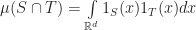
, then the shapes collide.  One way to compute this volume is to rewrite it as an integral.  Let 1_S denote the indicator function of S, then

\mu(S \cap T) = \int \limits_{\mathbb{R}^d} 1_S(x) 1_T(x) dx

This integral is essentially a dot product.  If we perform an expansion of 1_S, 1_T in some basis, (for example, as Fourier waves), then we can use that to approximate this volume.  If we do this expansion carefully, then with enough work we can show that the resulting approximation preserves something of the original geometry.  For more details, here is a paper I wrote:

M. Lysenko, (2013) “Fourier Collision Detection” International Journal of Robotics Research

The advantage to this type of approach to collision detection is that it can support any sort of geometry, no matter how complicated. This is because the cost of the testing intersections scales with the accuracy of the collision test in a predictable, well-defined way.  The disadvantage though is that at high accuracies it is slower than other exact techniques.  Whether it is worthwhile or not depends on the desired accuracy, the types of shapes involved and if additional information like a separating axis is needed and so on.

Broad phase

Given a fast narrow phase collision test, we can solve the broad phase collision detection problem for n objects in O(n^2) calls to the underlying test.  As the number of reported collisions could be O(n^2) in the worst case, this would seem optimal.  However, we can get a sharper picture using a more detailed output sensitive analysis.  To do this, define k to be the number of reported intersections, and let us then analyze the time required to do the collision detection as a function of both n and k.  Using output sensitive analysis, there is also a lower bound of \Omega(n \log(n) + k) (for comparison based algorithms) by reduction to the element uniqueness problem.

Special cases

If we are only allowed to use pairwise intersection tests and know no other property of the shapes, then it is impossible to compute all pairwise intersections any faster than O(n^2 + k).  However, for special types of shapes in low dimensional spaces substantially faster algorithms are known:

Line segments

For line segments in the plane, it is possible to report all intersections in O((n+k) \log(n)) time using a sweep line algorithm.  If k \in o( \frac{n^2}{\log(n)} ), this is a big improvement over naive brute force.  This technique can also be adapted to compute intersections in sets of general convex polygons by decomposing them into segments, and then building a secondary point location data structure to handle the case where a polygon is completely contained in another.

Uniformly sized and distributed balls

It is also possible to find all intersections in a collection of balls with constant radii in optimal O(n + k) time, assuming that the number of balls any single ball intersects is at most O(1).  The key to this idea is to use a grid, or hash table to detect collisions. This process is both simple to implement and has robust performance, and so it is used in many simulations and video games.

Axis aligned boxes

Finally, it is possible to detect all intersections in a collection of axis aligned boxes in O(n \log^d(n) + k) time, though we will postpone talking about this until next time.

General objects and bounding volumes

For general objects, no algorithms with running time substantially faster than O(n^2 + k) are known.  However, we can in practice still get a big speed up by using a simpler broad phase collision test to filter out intersections.  The main idea is to cover each object, S, with some simpler shape S' \supseteq S called a bounding volume.  If a pair of bounding volumes do not intersect, then the shapes which they are covering can not intersect either.  In this way, bounding volumes can be used to prune down the set of collision tests which must be performed.

In practice, the most common choice for a bounding volume is either a box or a sphere.  The reason for this is that boxes and spheres support efficient broad phase intersection tests, and so they are relatively cheap.

Spheres tend to be more useful if all of the shapes are more or less the same size, but computing tight bounding spheres is slightly more expensive.  For example, if the objects being intersected consist of uniformly subdivided triangle meshes, then spheres can be a good choice of bounding volume.  However, spheres do have some weakness.  Because testing sphere intersection requires multiplication, it is harder to do it exactly than it is for boxes.  Additionally, for spheres of highly variable sizes it is harder to detect intersections efficiently.

Computing intersections in boxes on the other hand tends to be much cheaper, and it is simpler to exactly detect if a pair of boxes intersect.  Also for many shapes boxes tend to give better approximations than spheres, since they can have skewed aspect ratios.  Finally, broad phase box intersection has theoretically more robust performance than sphere intersection for highly variable box sizes.  Perhaps based on these observations, it seems that most modern high performance physics engines and intersection codes have converged on axis-aligned boxes as the preferred primitive for broad phase collision detection.  (See for example, Bullet, Box2D)

Bipartite vs complete

It is sometimes useful to separate objects for collision detection into different groups.  For example if we are intersecting water-tight meshes, it is useless to test for self intersections.  Or as another example, in a shooter game we only need to test the player’s bullets against all enemies.  These are both examples of bipartite collision detection.  In bipartite collision detection, we have two groups of objects (conventionally colored red and blue), and the goal is to report all pairs of red and blue objects which intersect.

Range searching and more references

There is a large body of literature on intersection detection and the related problems of range searching.  Agarwal and Erickson give an excellent survey of these results in the following paper,

P.K. Agarwal, J. Erickson. (1997) “Geometric range searching and its relatives

Next time

In the next article, we will look at broad phase collision detection in more depth, focusing on boxes as a basic primitive.