0 FPS

In the last two posts I introduced ndarrays, and explained the rationale and implementation details of the library.  In this post I am going to show a few of the libraries that I have written using ndarrays.  All of this code works in both node.js and within any browser that supports typed arrays.  You can run the demos directly in node.js or else test them out in a browser using a bundler like browserify.  You can click on the links for each of them to find out more details about a specific module.

Vector arithmetic

cwise: Array operation meta-programming library

ndarray-ops: Common array operations

ndarray-complex: Array operations for complex numbers

Image processing

get-pixels: Reads the pixels from an image as an ndarray

save-pixels: Writes a 2D ndarray to an image file

lena: The Lena test image as a require()able commonjs module.

luminance: Converts an rgb image into luminance.

normalize: Scales an ndarray to mean 0 and standard deviation 1

ndarray-warp: Apply a non-linear warp to an ndarray

Fourier analysis

ndarray-fft: Fast fourier transform for ndarrays

ndarray-convolve: Convolutions and correlations for ndarrays

phase-align: Pattern matching and alignment

ndarray-translate-fft: Phase shifts an ndarray

Morphology and miscellaneous stuff

ndarray-pack: Convert a numeric.js array to an ndarray

ndarray-moments: Calculate first few terms of moment generating function

distance-transform: Fast distance transforms

ball-morphology: Mathematical morphology with ball-shaped structuring elements

Conclusions

This list is by no means exhaustive, and I have been writing more modules as I need them.  One of the nice things about working with CommonJS modules is that it is pretty straight forward to create your own module on npm, and reuse its functionality.  I think that this style of programming could make building large scientific computing projects like SciPy/NumPy much more manageable.  Each function in such a project could be decomposed into a separate module, and it would be easy to experiment with different implementations.

I must confess that secretly the article I wrote last time (in which I introduced ndarrays) was just a pretext to introduce the stuff that I am going to write about today: which is the cwise library for array operations in JavaScript.

Array operations

Briefly, array operations are component-wise operations that can be applied across multiple multidimensional arrays simultaneously.  Array operations can be used to implement basic vector arithmetic, like addition or scaling and are a fundamental tool in linear algebra/numerical computing in general.  Because they are so ubiquitous, many languages have special syntax for array operations as well as routines for specifically optimizing the performance; for example in MATLAB if you prefix an operator with . then executes component-wise.  In the functional programming world, array operations can be implemented as a sequence of zip /map /reduce higher order functions, while in a language with procedural constructs like C or JavaScript you would probably just use a for-loop like this:

for(i=0; i<shape[0]; ++i) {
 for(j=0; j<shape[1]; ++j) {
   // ... do operation ...
   a[i][j] += b[i][j]
 }
}

The goal of this article is to investigate different ways to implement these sorts of array operations across multiple ndarrays of various shapes and strides.

Simple algorithm

The simple for-loop algorithm is a good starting point for implementing operations on ndarrays.  However, in an ndarray performing a lookup at each loop iteration introduces an overhead of (where is the dimension  of the ndarray) due to the extra indexing and multiplication required.  To avoid doing this, we can compute the index into the underlying array incrementally.  As a sketch of how this works, consider the following psuedocode:

var a_ptr = a.offset
  , b_ptr = b.offset

for(var i=0; i<a.shape[0]; ++i) {
  for(var j=0; j<a.shape[1]; ++j) {
    //... do operation ...
    a.data[a_ptr] += b.data[b_ptr]

    //Advance pointers along axis 1:
    a_ptr += a.stride[1]
    b_ptr += b.stride[1]
  }
  //Advance pointers along axis 0:
  a_ptr += a.stride[0] - a.stride[1] * a.shape[1]
  b_ptr += b.stride[0] - b.stride[1] * a.shape[1]
}

Using this new algorithm, the next index for the arrays can be computed by just adding some constant shift to the pointer instead of performing a series of multiplies.  This is indeed a good thing, and one can easily show that in the conventional RAM model of computation, (which is heavily emphasized in undergraduate CS curricula), this approach is optimal.

But as everyone who has ever tried hard to optimize code for processing arrays knows, this is hardly the full story.  Real computers have hierarchical memory, and execute block IO operations on chunks of cache.  Failing to take this into account when analyzing an algorithm can lead to wildly different (and inaccurate) conclusions about its performance.

Two-level memory and striding

So if we want to come up with a better algorithm for array operations we need a better theory of how our computer works.  And perhaps the simplest extension of the RAM model which does this is the two-level memory model.  The basic idea in the two-level model is that you are allowed to operate on memory in contiguous chunks of up to size words at a time.  This is basically a block IO version of the RAM model, and accurately models many realistic algorithms.  In general, the running time of an algorithm on the RAM model is an upper bound on its running time in the two-level model, and the fastest that we can ever speed up an algorithm in the two level model is by a factor of .

This fact is especially important when we are considering array operations and illustrates the importance of striding in our algorithms.  For example, suppose in the above algorithm that the arrays were contiguously packed in row major order, then each of the memory reads could be executed sequentially and the running time would be .  On the other hand, if the arrays were stored in column major order and if we looped over them in the same order, then we would get no advantage from blocked IO operations and so the cost of executing the algorithm would be .

To fix this, we should iterate over the indices where the largest strides are in the outer loop and the smallest strides are packed inside.  This makes the most efficient use of each block memory operation, and reduces the total computation time by a factor of (which is optimal) if the stride orderings are compatibile in each array.

Cache aware algorithm

So the next question is what happens if the strides are not compatible?  For example, suppose that a was column major while b was row major?  Then in the two level model there is no way to take advantage of block memory operations to speed up our loop, and so it would seem that we are back to RAM model performance.  However, there is an important aspect of hierarchical memory which the two level model neglects: caching.

But before we can understand and exploit this new technology, we need some sort of model to describe how it works.  For this purpose, the minimal extension of the two level  memory model is known as the external memory model.  Like the two level memory model, we can read and write memory in chunks, but in addition there is also a separate (but small and finite) memory called the cache which can store up to words at a time.  We assume that accessing cache is infinitely fast, and so the time complexity of any algorithm in the external memory model is bounded by the number of reads/writes to the external memory source.

This model may seem slightly absurd since it is possible to execute things like infinite loops for free (as long as they only use the cache), however it turns out to be pretty good accurate for numerical computations and data structures, which are all asymptotically limited by the amount of time they spend moving bits around at the slowest level of the memory hierarchy.

Now it turns out that within the external memory model there is an asymptotically efficient algorithm for array operations that works regardless of their stride.  The first place where this seems to have been written down is in the following paper:

A. Aggarwal, J. Vitter. “The input/output complexity of sorting and related problems” (1987) CACM

The general idea is that we break our arrays down into chunks which have shapes that are on the order of in each dimension.  Then we iterate over the whole matrix in these chunks and execute the array operation across each chunk independently.  In psuedocode, it works like this:

//Assume shape[0], shape[1] are multiples of B for simplicity
for(var i=0; i<shape[0]; i+=B) {
  for(var j=0; j<shape[1]; j+=B) {
    var a_ptr = i * a.stride[0] + j * a.stride[1]
    var b_ptr = i * b.stride[0] + j * b.stride[1]
    for(var k=0; k<B; ++k) {
      for(var l=0; l<B; ++l) {
        a.data[a_ptr] += b.data[b_ptr]
        a_ptr += a.stride[1]
        b_ptr += b.stride[1]
      }
      a_ptr += a.stride[0] - a.stride[1] * B
      b_ptr += b.stride[0] - b.stride[1] * B
    }
  }
}

Now if , then this approach can be used to speed up any array operation by a factor – regardless of their stride!  Pretty neat!

Cache oblivious algorithm

The above approach is awesome, but it only works if we know how big and are.  However, how can we figure out what these parameters are?  One possible solution is to run lots of experiments and directly optimize those values.  This benchmark-first approach to performance tuning works pretty well for known hardware configurations, like game consoles or iPhone and can produce awesome results.  However it is obviously not very robust, nor is it even feasible in all situations, like web applications for example which need to perform well across many different browsers and devices.  

Similarly, we often can’t count on the values for and to remain constant throughout the life time of a program.  Contention for disk, RAM and CPU cache can cause the amount of available cache and bandwidth to fluctuate, and so we really shouldn’t assume these things are constant.

Finally, there is also the small problem that computers typically have more than one level of caching, and optimizing array operations for multiple levels of cache would require introducing one extra loop per layer, which can be quite impractical to implement.

Fortunately there is a single elegant model of computation which solves all of these problems at once.  It is known as the cache oblivious memory model, and it was invented by Harald Prokop:

H. Prokop. “Cache-oblivious algorithms” (1999) MIT Master’s Thesis.

For the amount of problems that it solves, the cache oblivious model of computation is remarkably simple: it is just the external memory model, except we are not allowed to know and .  But despite being so trivial, the cache oblivious model has a number of remarkable properties:

1. Algorithms that scale in the cache oblivious model scale across all levels of the memory hierarchy simultaneously.
2. Cache oblivious algorithm “just work” across any type of hardware or virtual machine with no fine tuning.
3. Cache oblivious algorithms automatically throttle with hardware availability and scale performance accordingly.
4. Finally, programs written for the cache oblivious model look just like ordinary RAM model programs!  There is no need to introduce extra notation or operations.

These properties make the cache oblivious model the gold standard for analyzing high performance algorithms, and it should always be our goal to design data structures and algorithms that scale in this model.  However, to achieve these benefits we need to do a bit more work up front when we are designing our algorithms.

For array operations, a simple way to do this is to adapt Prokop’s cache oblivious matrix transpose algorithm (see the above thesis for details).  The way it works is that we keep recursively splitting our multidimensional arrays in half along the largest axis until finally we are left with blocks of unit size.  In psuedo-JavaScript using ndarrays, it would look like this:

function recursiveAdd(a, b) {
  var rows = a.shape[0]
    , cols = a.shape[1]
  if(rows === 1 && cols === 1) {
    a.data[a.offset] += b.data[b.offset]
  } else if(rows > cols) {
    rows >>>= 1
    recursiveAdd(a.hi(rows, cols), b.hi(rows, cols))
    recursiveAdd(a.lo(rows, 0), b.lo(rows, 0))
  } else {
    cols >>>= 1
    recursiveAdd(a.hi(rows, cols), b.hi(rows, cols))
    recursiveAdd(a.lo(0, cols), b.lo(0, cols))
  }
}

The above code also works regardless of the stride and always uses an optimal block memory transfers if the cache is at least .  It is also pretty easy to generalize this idea to multiple arrays with higher dimensions, which again performs optimally assuming that where n is the number of arguments and d is the dimension of the arrays.

Array operations for JavaScript

The above cache oblivious algorithm is clearly what we want to implement, but the code in the previous listing is just a sketch and if implemented naively is not likely to be very fast (at least in JavaScript).  There are quite a few important JS-specific micro-optimizations that we ought to apply before seriously implementing cache-oblivious array operations:

• Slicing the arrays creates a small amount of garbage at each level of recursion, and so we should probably flatten out the objects and keep track of their structures as arguments incrementally to avoid unnecessary memory allocation.
• Using a recursive function call is much slower than manually using a stack to keep track of previous calls,.
• Similarly, we should use the pointer tricks from the simple algorithm to speed up array indexing.
• Also if the strides match, we should use the direct pointer arithmetic version as it has lower overhead
• For small array sizes the overhead of recursion is much larger than the savings due to cache improvements, and so we would want to terminate the subdivision sometime before getting all the way down to unit arrays.  (This is not related to the size of the cache blocks since it is a function of the amount of CPU overhead, not memory bandwidth).

Code!

All of these issues can be pretty tricky to get right, and so it makes sense to try to push all of this complexity into a library.  This is what the cwise library does, and you can get it here:

https://github.com/mikolalysenko/cwise

That library should work in any JavaScript environment that supports typed arrays, including most current browsers (IE 9+, Firefox, Chrome and Safari).  If you want to try it out in your own projects, you can install it via npm or use browserify (or some similar tool) to stick it in your web page.

Macros and dynamic code generation

The basic idea behind cwise is similar to libraries like FFTW which dynamically generate tuned code based on their inputs (though because it is much easier to do dynamic code generation in JavaScript the interface for cwise is a bit simpler).  The way it works is that it lazily compiles optimized scans for array operations based on the shape and stride of the input arguments.  You can specify the component-wise operations for cwise using ordinary JavaScript which gets parsed and compiled using esprima/falafel at run time.  This is only done the first time you execute a cwise function, all subsequent calls reuse the same optimized script.

Tricks

There are a lot of useful things that you can do with ndarrays using cwise.  There are plenty of useful recipes on the github page, but to help get things started here is a quick survey of some stuff you can do:

Vector arithmetic

The most obvious use of cwise is to implement basic vector arithmetic.  You can grab a handful of prebaked ready-to-go operations from the following github project:

https://github.com/mikolalysenko/ndarray-ops

As a rule, using these sort of helper methods is not as efficient as unpacking your array operations into a cwise data structure, but on the other hand they can simplify your code and for basic tasks they are often fast enough.

Matrix transpose

A more complicated example of using ndarrays is to perform matrix transpose or cache oblivious reindexing of arrays.  For example, this is pretty easy to do by just changing the stride in the target.  Suppose for example, suppose we want to transpose a square image which is stored in column-major format.  Then we can do this using the following code:

var ops = require("ndarray-ops")
var ndarray = require("ndarray")
function transpose(output, input, size) {
  var a = ndarray.ctor(output, [size, size], [size, 1], 0)
    , b = ndarray.ctor(input, [size, size], [1, size], 0)
  ops.assign(a, b)
}

This is essentially the same thing that Prokop’s cache oblivious matrix transpose algorithm does.

Array copying

Another neat trick we can do with array operations is make copies of arrays in memory.  For example, if we want to fill an array with a repeating pattern, we can use the following snippet:

var ops = require("ndarray-ops")
var ndarray = require("ndarray")
function fillPattern(output, pattern, count) {
  var a = ndarray.ctor(output, [count, pattern.length], [pattern.length, 1], 0)
    , b = ndarray.ctor(pattern, [count, pattern.length], [0, 1], 0)
  ops.assign(a, b)
}

This generalizes to filling 2D images with repeated tiles or for stuff like slicing volume data apart into a texture.

Experiments

So how much difference does all of this make?  To add some numbers to all of these different array operations I made a few quick experiments in node.js to try everything out.  You can check out the results for yourself here on github:

https://github.com/mikolalysenko/cwise-experiment

And here are the results summarized in graphical format:

We can draw the following conclusions from these measurements:

• When possible, sequential iteration is the optimal implementation of array operations.
• For non-compatible strides, cache aware array operations are fastest, but they require knowledge of the underlying architecture (which may not always be available)
• Though cache oblivious array operations are almost never the fastest possible algorithm, they come closest across the widest array of possible inputs.

Conclusion

In summary, we’ve discussed an asymptotically optimal algorithm cache-oblivious array operations across many multidimensional arrays with arbitrary shapes and strides.  We’ve also seen an implementation of these concepts in JavaScript via the ndarray and cwise libraries (that should work in node.js and in any browser that supports typed arrays).  These tools enable a wide variety of interesting image processing and linear algebra operations, but a lot more work is still necessary to realize a full suite of numerical linear algebra tools in JavaScript.  Here are a few possible ideas for future projects:

• Tools for basic linear algebra computations (matrix inverse, iterative/direct solvers, eigenvalue problems)
• Data structures for sparse multidimensional arrays
• Libraries for implementing Einstein tensor summation/higher order map-reduce in a style similar to cwise.

The past few months I’ve been working to move more of my work into JavaScript, and in particular the node.js ecosystem.  I hope that by doing this I will be able to create better demos and applications that are easier to use as well as develop.

Numerical Computing in a Hostile Environment

But despite the numerous practical advantages to working in JavaScript (especially from a user experience perspective) there are still many things that JS just sucks at.  For me the most painful of these is the weak support for numerical computing and binary data types.  These problems are due to fundamental limitations of the language, and not something that can be papered over in a library.  For example, in JS there is:

• No pass-by-value for non-primitive data types
• No way to control memory alignment for members of objects
• No way to restrict references to pointers/prevent aliasing
• No way to ensure arrays of objects are allocated in place
• No operator overloading
• No array operations
• No SIMD instructions and data types
• … etc.

This situation is bad, but the benefits of using JS from an accessibility perspective are just too big to ignore, and so it is at least worth it to try as much as can be done within the limitations of the system.  Moreover, these obstacles are by no means unprecedented in the world of computing.  As an instructive example, consider the Java programming language:  Java suffers from exactly the same design flaws listed above, and yet it is a viable platform for numerical computing with an enthusiastic community (though it is still nowhere near as fast as more efficiently designed languages like Fortran/C99).  So, it is a plausible hypothesis that JavaScript could achieve similar results.

Now, reimplementing say LAPACK or SciPy is a huge project, and it is not reasonable to try doing it in a single article or even within a single library.  To help focus our inquiries, let us first restrict the scope of our search.    Instead, let us study today on the fundamental problem of implementing multidimensional arrays.

Multidimensional arrays

Multidimensional arrays are a natural first step towards building systems for solving numerical problems, and are a generally useful data type in their own right, with applications in graphics and vision.  In a language like JavaScript, there are multiple ways 

Arrays-of-Arrays

Perhaps the most popular way to represent higher dimensional arrays in JavaScript is as arrays-of-arrays.  For example,

var A = [[1, 0, 0],
         [0, 1, 0],
         [0, 0, 1]]

This is the approach that numeric.js uses, and it has some merits.  For example, the syntax for accessing elements in an array-of-arrays is quite pleasingly simple:

var x = A[i][j]

And it does not require introducing any extra data structures or conventions into the language.

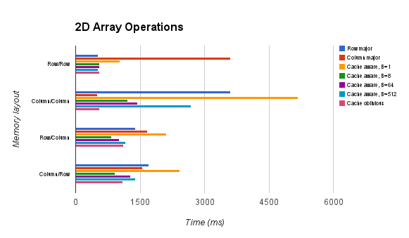
However, while arrays-of-arrays are by far the simplest solution, from a performance perspective they are disastrous.  The most obvious problem is that to allocate a d-dimensional array-of-arrays with O(n) elements per each element, you need to store extra bytes worth of memory in pointers and intermediate arrays.  Additionally, accessing an element in an array-of-arrays requires dependent memory dereferences.  These operations can’t be easily pipelined and are terrible from a cache performance perspective.  If performance is even remotely close to being an objective, then we need to try for something better.

Typed Arrays

Fortunately, in both JavaScript and Java, there is a better alternative to arrays-of-arrays: namely typed arrays.  Using a typed array lets us guarantee that the data for our array is arranged contiguously with no wasted space.  For example, here is how we would create a typed array for the same matrix described earlier:

var A = new Float32Array([1, 0, 0, 0, 1, 0, 0, 0, 1])

The downside is that accessing elements from a typed array is a bit more complicated.  To do this we need to agree on some convention up front about how the elements in the array are arranged in memory.  In languages like C, typically this is done in colexicographic (also known as row major order), while other languages like Fortran use a lexicographic ordering (also called column major order).  The choice between the two is  totally arbitrary, but once you pick one you have to stick with it.  Assuming a row major ordering then, we can access an element from the array using the formula:

var x = A[3 * i + j]

Typed arrays can be very fast, but they are a bit clumsy to work with.  You need to keep track of the number of both what convention you are using to store the array as well as what its dimensions are, which is an extra blob of data that needs to be passed around and slows things down substantially.

Strided Arrays

Strided arrays solve these problems by considering array storage in a more general form. Instead of keeping a fixed convention for indexing, they write the index of an element in array as a general linear function of its coordinate.  For example,

var x = A[ c0 * i + c1 * j + ... ]

The result is that they achieve the same performance as flattened typed arrays, but gain the advantage that they can be easily sliced, transposed or reversed just by changing the stride.  For example, if we wanted to switch the x/y axes of an image, all that we would need to do is swap the strides:

var x = A[ c1 * i + c0 * j + ... ]

Setting a stride to a negative value can be used to reverse an axis, and changing the shape of an array lets us easily crop out subarrays from higher dimensional arrays.

Introducing ndarray

At least theoretically, strided arrays sound like a great idea and so to see how well they worked in practice I created the following library:

https://github.com/mikolalysenko/ndarray

Essentially, an ndarray is an object that has 4 pieces of data:

• data – The underlying typed array
• shape – The shape of the ndarray
• stride  – The stride of the ndarray
• offset – A pointer to the first element in the array

To look up an item in an ndarray you use the formula:

data[stride[0] * i[0] + stride[1] * i[1] + ... + offset]

You can download it and try it out yourself using npm, or check out some projects already built on top of ndarray here.

But is it fast?

To see how each of these multidimensional array representations compare, I decided to compare their performance on a simple component-wise operation for various shapes of arrays.  In pseudocode, this operation looks something like:

function test(A, B) {
  for(i in range) {
    A[i] += B[i] + 0.1
    B[i] -= A[i] * 0.5
  }
}

I ran this simple loop using different variations of multidimensional arrays with various shapes.  The following chart summarizes the results:

You can find more detailed results and further experiments (including direct comparisons using numeric.js) at the github page for this project:

https://github.com/mikolalysenko/ndarray-experiments

These results are somewhat typical, indexing in an ndarray is a little slower than directly walking over a typed array, but not by much.  For arrays of arrays, the performance gets progressively worse as the first axes get larger, but even in the best case they trail far behind data structures built on typed arrays.

Next time

The natural question to ask is can we do even better?  And the answer is yes.  The key to getting further performance improvements is to batch operations together allowing for full array comprehensions.  I’ll discuss this in the next post, but for now you can take a look at my current implementation of bulk operations on ndarrays in the cwise library.

This is a post about a silly (and mostly pointless) optimization.  To motivate this, consider the following problem which you see all the time in mesh processing:

Given a collection of triangles represented as ordered tuples of indices, find all topological duplicates.

By a topological duplicate, we mean that the two faces have the same vertices.  Now you aren’t allowed to mutate the faces themselves (since orientation matters), but changing their order in the array is ok.  We could also consider a related problem for edges in a graph, or for tetrahedra in mesh.

There are of course many easy ways to solve this, but in the end it basically boils down to finding some function or other for comparing faces up to permutation, and then using either sorting or hashing to check for duplicates.  It is that comparison step that I want to talk about today, or in other words:

How do we check if two faces are the same?

In fact, what I really want to talk about is the following more general question where we let the lengths of our faces become arbitrarily large:

Given a pair of arrays, A and B, find a total order such if and only if up to some permutation .

For example, we should require that:

[0, 1, 2] [2, 0, 1]

[2, 0, 1] [0, 1, 2]

And for two sequences which are not equal, like [0,1,2] and [3, 4, 5] we want the ordering to be invariant under permutation.

Obvious Solution

An obvious solution to this problem is to sort the arrays element-wise and return the result:

function compareSimple(a, b) {
  if(a.length !== b.length) {
    return a.length - b.length;
  }
  var as = a.slice(0)
    , bs = b.slice(0);
  as.sort();
  bs.sort();
  for(var i=0; i<a.length; ++i) {
    var d = as[i] - bs[i];
    if(d) {
      return d;
    }
  }
  return 0;
}

This follows the standard C/JavaScript convention for comparison operators, where it returns -1 if a comes before b, +1 if a comes after b and 0 if they are equal.  For large enough sequences, this isn’t a bad solution.  It takes time and is pretty straightforward to implement.  However, for smaller sequences it is somewhat suboptimal.  Most notably, it makes a copy of a and b, which introduces some overhead into the computation and in JavaScript may even trigger a garbage collection event (bad news).  If we need to do this on a large mesh, it could slow things down a lot.

An obvious way to fix this would be to try inlining the sorting function for small values of n (which is all we really care about), but doing this yourself is pure punishment.  Here is an `optimized` version for length 2 sets:

function compare2Brutal(a, b) {
  if(a[0] < a[1]) {
    if(b[0] < b[1]) {
      if(a[0] === b[0]) {
        return a[1] - b[1];
      }
      return a[0] - b[0];
    } else {
      if(a[0] === b[1]) {
        return a[1] - b[0];
      }
      return a[0] - b[1];
    }
  } else {
    if(b[0] < b[1]) {
      if(a[1] === b[0]) {
        return a[0] - b[1];
      }
      return a[1] - b[0];
    } else {
      if(a[1] === b[1]) {
        return a[0] - b[0];
      }
      return a[1] - b[1];
    }
  }
}

If you have any aesthetic sensibility at all, then that code probably makes you want to vomit.   And that’s just for length two arrays!  You really don’t want to see what the version for length 3 arrays looks like.  But it is faster by a wide margin.  I ran a benchmark to try comparing how fast these two approaches were at sorting an array of 1000 randomly generated tuples, and here are the results:

• compareSimple:  5864 µs
• compareBrutal: 404 µs

That is a pretty good speed up, but it would be nice if there was a prettier way to do this.

Symmetry

The starting point for our next approach is the following screwy idea:  what if we could find a hash function for each face that was invariant under permutations?  Or even better, if the function was injective up to permutations, then we could just use the `symmetrized hash` compare two sets.  At first this may seem like a tall order, but if you know a little algebra then there is an obvious way to do this; namely you can use the (elementary) symmetric polynomials.  Here is how they are defined:

Given a collection of numbers, the kth elementary symmetric polynomial, is the coefficient of in the polynomial:

For example, if , then the symmetric polynomials are just:

And for we get:

The neat thing about these functions is that they contain enough data to uniquely determine up to permutation.  This is a consequence of the fundamental theorem for elementary symmetric polynomials, which basically says that these polynomials form a complete independent basis for the ring of all symmetric polynomials.  Using this trick, we can formulate a simplified version of the sequence comparison for :

function compare2Sym(a, b) {
   var d = a[0] + a[1] - b[0] - b[1];
   if(d) {
     return d;
   }
   return a[0] * a[1] - b[0] * b[1];
}

Not only is this way shorter than the brutal method, but it also turns out to be a little bit faster.  On the same test, I got:

• compare2Sym: 336 µs

Which is about a 25% improvement over brute force inlining.  The same idea extends to higher n, for example here is the result for :

function compare3Sym(a, b) {
  var d = a[0] + a[1] + a[2] - b[0] - b[1] - b[2];
  if(d) {
    return d;
  }
  d = a[0] * a[1] + a[0] * a[2] + a[1] * a[2] - b[0] * b[1] - b[0] * b[2] - b[1] * b[2];
  if(d) {
    return d;
  }
  return a[0] * a[1] * a[2] - b[0] * b[1] * b[2];
}

Running the sort-1000-items test against the simple method gives the following results:

• compareSimple: 7637 µs
• compare3Sym:  352 µs

Computing Symmetric Polynomials

This is all well and good, and it avoids making a copy of the arrays like we used in the basic sorting method.  However, it is also not very efficient.  If one were to compute the coefficients of a symmetric polynomial directly using the naive method we just wrote, then you would quickly end up with terms!  That is because the number of terms in , and so the binomial theorem tells us that:

A slightly better way to compute them is to use the polynomial formula and apply the FOIL method.  That is, we just expand the symmetric polynomials using multiplication.  This dynamic programming algorithm speeds up the time complexity to .  For example, here is an optimized version of the case:

function compare3SymOpt(a,b) {
  var l0 = a[0] + a[1]
    , m0 = b[0] + b[1]
    , d  = l0 + a[2] - m0 - b[2];
  if(d) {
    return d;
  }
  var l1 = a[0] * a[1]
    , m1 = b[0] * b[1];
  d = l1 * a[2] - m1 * b[2];
  if(d) {
    return d;
  }
  return l0 * a[2] + l1 - m0 * b[2] - m1;
}

For comparison, the first version of compare3 used 11 adds and 10 multiplies, while this new version only uses 9 adds and 6 multiplies, and also has the option to early out more often.  This may seem like an improvement, but it turns out that in practice the difference isn’t so great.  Based on my experiments, the reordered version ends up taking about the same amount of time overall, more or less:

• compare3SymOpt: 356 µs

Which isn’t very good.  Part of the reason for the discrepancy most likely has something to do with the way compare3Sym gets optimized.  One possible explanation is that the expressions in compare3Sym might be easier to vectorize than those in compare3SymOpt, though I must admit this is pretty speculative.

But there is also a deeper question of can we do better than asumptotically?  It turns out the answer is yes, and it requires the following observation:

Polynomial multiplication is convolution.

Using a fast convolution algorithm, we can multiply two polynomials together in time.  Combined with a basic divide and conquer strategy, this gives an algorithm for computing all the elementary symmetric functions. However, this is still worse than sorting the sequences!  It feels like we ought to be able to do better, but further progress escapes me.  I’ll pose the following question to you readers:

Question: Can we compute the n elementary symmetric polynomials in time or better?

Overflow

Now there is still a small problem with using symmetric polynomials for this purpose: namely integer overflow.  If you have any indices in your tuple that go over 1000 then you are going to run into this problem once you start multiplying them together.  Fortunately, we can fix this problem by just working in a ring large enough to contain all our elements.  In languages with unsigned 32-bit integers, the natural choice is , and we get these operations for free just using ordinary arithmetic.

But life is not so simple in the weird world of JavaScript!  It turns out for reasons that can charitably be described as “arbitrary” JavaScript does not support a proper integer data type, and so every number type in the language gets promoted to a double when it overflows whether you like it or not (mostly not).  The net result:  the above approach messes up.  One way to fix this is to try applying a modulus operator at each step, but the results are pretty bad.  Here are the timings for a modified version of compare2Sym that enforces bounds:

• compare2Masked: 1750 µs

That’s more than a 5-fold increase in running time, all because we added a few innocent bit masks!  How frustrating!

Semirings

The weirdness of JavaScript suggests that we need to find a better approach.  But in the world of commutative rings, it doesn’t seem like there are any immediately good alternatives.  And so we must cast the net wider.  One interesting possibility is to extend our approach to include semirings.  A semiring is basically a ring where we don’t require addition to be invertible, hence they are sometimes called “rigs” (which is short for a “ring without negatives”, get it? haha).

Just like a ring, a semiring is basically a set with a pair of operators that act as generalized addition and multiplication.  You also have a pair of elements, which act as the additive and multiplicative identity.  These things then have to satisfy a list of axioms which are directly analogous to those of the natural numbers (ie nonnegative integers).  Here are a few examples of semirings, which you may or may not be familiar with:

• The complex numbers are semiring (and more generally, so is every field)
• The integers are a semiring (and so is every other ring)
• The natural numbers are a semiring (but not a ring)
• The set of Boolean truth values, under the operations OR, AND is a semiring (but is definitely not a ring)
• The set of reals under the operations min,max is a semiring (and more generally so is any distributive lattice)
• The tropical semiring, which is the set of reals under (max, +) is a semiring.

In many ways, semirings are more fundamental than rings.  After all, we learn to count stuff using the natural numbers long before we learn about integers.  But they are also much more diverse, and some of our favorite definitions from ring theory don’t necessarily translate well.  For those who are familiar with algebra, probably the most shocking thing is that the concept of an ideal in a ring does not really have a good analogue in the language of semirings, much like how monoids don’t really have any workable generalization of a normal subgroup.

Symmetric Polynomials in Semirings

However, for the modest purposes of this blog post, the most important thing is that we can define polynomials in a semiring (just like we do in a ring) and that we therefore have a good notion of an elementary symmetric polynomial.  The way this works is pretty much the same as before:

Let be a semiring under ; then we have the symmetric functions.  Then for two variables, we have the symmetric functions:

And for we get:

And so on on…

Rank Functions and (min,max)

Let’s look at what happens if we fix a particular semiring, say the (min,max) lattice.  This is a semiring over the extended real line where:

• 
• 
• 
• 

Now, here is a neat puzzle:

Question: What are the elementary symmetric polynomials in this semiring?

Here is a hint:

And…

Give up?  These are the rank functions!

Theorem: Over the min,max semiring, is the kth element of the sorted sequence

In other words, evaluating the symmetric polynomials over the min/max semiring is the same thing as sorting.  It also suggests a more streamlined way to do the brutal inlining of a sort:

function compare2Rank(a, b) {
  var d = Math.min(a[0],a[1]) - Math.min(b[0],b[1]);
  if(d) {
    return d;
  }
  return Math.max(a[0],a[1]) - Math.max(b[0],b[1]);
}

Slick!  We went from 25 lines down to just 5.  Unfortunately, this approach is a bit less efficient since it does the comparison between a and b twice, a fact which is reflected in the timing measurements:

• compare2Rank: 495 µs

And we can also easily extend this technique to triples as well:

function compare3Rank(a,b) {
  var l0 = Math.min(a[0], a[1])
    , m0 = Math.min(b[0], b[1])
    , d  = Math.min(l0, a[2]) - Math.min(m0, b[2]);
  if(d) {
    return d;
  }
  var l1 = Math.max(a[0], a[1])
    , m1 = Math.max(b[0], b[1]);
  d = Math.max(l1, a[2]) - Math.max(m1, b[2]);
  if(d) {
    return d;
  }
  return Math.min(Math.max(l0, a[2]), l1) - Math.min(Math.max(m0, b[2]), m1);
}

• compare3Rank: 618.71 microseconds

The Tropical Alternative

Using rank functions to sort the elements turns out to be much simpler than doing a selection sort, and it is way faster than calling the native JS sort on small arrays while avoiding the overflow problems of integer symmetric functions.  However, it is still quite a bit slower than the integer approach.

The final method which I will now describe (and the one which I believe to be best suited to the vagaries of JS) is to compute the symmetric functions over the (max,+), or tropical semiring.  It is basically a semiring over the half-extended real line, with the following operators:

• 
• 
• 
• 

There is a cute story for why the tropical semiring has such a colorful name, which is that it was popularized at an algebraic geometry conference in Brazil.  Of course people have known about (max,+) for quite some time before that and most of the pioneering research into it was done by the mathematician Victor P. Maslov in the 50s.  The (max,+) semiring is actually quite interesting and plays an important role in the algebra of distance transforms, numerical optimization and the transition from quantum systems to classical systems.

This is because the (max,+) semiring works in many ways like the large scale limit of the complex numbers under addition and multiplication.  For example, we all know that:

But did you also know that:

This basically a formalization of that time honored engineering philosophy that once your numbers get big enough, you can start to think about them on a log scale.  If you do this systematically, then you eventually will end up doing arithmetic in the (max,+)-semiring.  Masolv asserts that this is essentially what happens in quantum mechanics when we go from small isolated systems to very big things.  A brief overview of this philosophy that has been translated to English can be found here:

Litvinov, G. “The Maslov dequantization, idempotent and tropical mathematics: a very brief introduction” (2006) arXiv:math/0501038

The more detailed explanations of this are unfortunately all store in thick, inscrutable Russian text books (but you can find an English translation if you look hard enough):

Maslov, V. P.; Fedoriuk, M. V. “Semiclassical approximation in quantum mechanics”

But enough of that digression!  Let’s apply (max,+) to the problem at hand of comparing sequences.  If we expand the symmetric polynomials in the (max,+) world, here is what we get:

And for :

If you stare at this enough, I am sure you can spot the pattern:

Theorem: The elementary symmetric polynomials on the (max,+) semiring are the partial sums of the sorted sequence.

This means that if we want to compute the (max,+) symmetric polynomials, we can do it in by sorting and folding.

Working the (max,+) solves most of our woes about overflow, since adding numbers is much less likely to go beyond INT_MAX.  However, we will tweak just one thing: instead of using max, we’ll flip it around and use min so that the values stay small.  Both theoretically and practically, it doesn’t save much but it gives us a maybe a fraction of a bit of extra address space to use for indices.  Here is an implementation for pairs:

function compare2MinP(a, b) {
  var d = a[0]+a[1]-b[0]-b[1];
  if(d) {
    return d;
  }
  return Math.min(a[0],a[1]) - Math.min(b[0],b[1]);
}

And it clocks in at:

• compare2MinP: 354 µs

Which is a bit slower than the symmetric functions, but still way faster than ranking.  We can also play the same game for :

function compare3MinP(a, b) {
  var l1 = a[0]+a[1]
    , m1 = b[0]+b[1];
  d = l1+a[2] - (m1+b[2]);
  if(d) {
    return d;
  }
  var l0 = Math.min(a[0], a[1])
    , m0 = Math.min(b[0], b[1])
    , d  = Math.min(l0, a[2]) - Math.min(m0, b[2]);
  if(d) {
    return d;
  }
  return Math.min(l0+a[2], l1) - Math.min(m0+b[2], m1);
}

Which hits:

• compare3MinP: 382 µs

Again, not quite as fast as integers, but pretty good for JavaScript.

Summary

You can get all the code to run these experiments on github:

https://github.com/mikolalysenko/set-compare

And here are the results that I got from running the experiment, all collated for easy reading:

Dimension = 2

• compareSimple: 5982 µs
• compare2Brutal: 415 µs
• compare2Sym: 352 µs
• compare2SymMasked: 1737 µs
• compare2Rank: 498 µs
• compare2MinP: 369 µs

Dimension = 3

• compareSimple: 7737 µs
• compare3Sym: 361 µs
• compare3Sym_opt: 362 µs
• compare3Rank: 612 µs
• compare3MinP: 377 µs

As you can see, the (min,+) solution is nearly as fast as the symmetric version without having the same overflow problems.

I hope you enjoyed reading this as much as I enjoyed tinkering around!  Of course I still don’t know of an optimal way to compare two lists.  As a final puzzle, I leave you with the following:

Question: Is there any method which can test if two unordered sequences are equal in linear time and at most log space?

Frankly, I don’t know the answer to this question and it may very well be impossible.  If you have any thoughts or opinions on this, please leave a comment!