Polynomials in C++

Last time, we showed how one can use symmetric tensors to conveniently represent homogeneous polynomials and Taylor series. Today, I am going to talk about how to actually implement a generic homogeneous polynomial/symmetric tensor class in C++. The goal of this implementation (for the moment) is not efficiency, but rather generality and correctness. If there is enough interest we can investigate some optimizations perhaps in future posts.

How to deal with polynomials?

There are quite a few ways to represent polynomials. For the moment, we aren’t going to assume any type of specialized sparse structure and will instead simply suppose that our polynomials are drawn at random from some uniform distribution on their coefficients. In some situations, for example in the solution of various differential equations, this is not too far from the truth, and while there may be situations where this assumption is too pessimistic, there are at least equally many situations where it is a good approximation of reality.

In 1D, the most direct method to represent a dense, inhomogeneous polynomial is to just store a big array of coefficients, where the $i^{th}$ entry corresponds to the coefficient for the degree i monomial. Naively generalizing a bit, the same idea works for multivariate polynomials as well, where you simply make the array multidimensional. For example, suppose you had the 2D coefficient matrix:

$\begin{array}{cc} a_{00} & a_{01} \\ a_{10} & a_{11} \end{array}$

Which we could then expand out to give a polynomial like:

$a_{00} + a_{01} x + a_{10} y + a_{11} xy$

Though it is a bit simplistic, working in this format does have a few advantages. For example:

Evaluating a polynomial is easy. Just compute the vectors $(1, x, x^2, ...), (1, y, y^2, ...)$ and the then plug them into the coefficient tensor using ordinary Einstein summation.
Multiplying can also be pretty fast. Observe that coefficient matrix of the product of two polynomial matrices is just the convolution of their two matrices. Using fast convolution algorithms (for example an FFT based method would work), this can be computed with only a mere log factor overhead!

The amount of storage for representing a polynomial on $d$ variables with a maximum per-coefficient degree of $r$ using this scheme requires exactly $(r+1)^d$ scalars worth of memory. However, this representation scheme does have some major problems:

It doesn’t capture all the terms above degree r properly. For example, if you take the term $a_{11} xy$ from the above example, it is actually second order, and so is the polynomial that it represents. However, we are missing the extra terms for $x^2, y^2$ .
Related to the previous point, it is not closed under linear coordinate transformations. If you were to say do a rotation in $x, y$ , that $a_{11} xy$ term could change into something like $a x^2 + b xy + c y^2$ , and thus we would need to resize the matrix to keep up with the extra stuff.
If you only care about storing terms with degree at most $r$ , then the above representation is wasteful by at least a factor of about $d!$ .
And if you want to deal with terms that are exactly degree d, then it is even worse with an overhead of $O( d! r^{ \frac{d}{d-1} })$ .

The underlying cause for each of these problems is similar, and ultimately stems from the fact that the function $M_{ij...} x^i y^j ...$ is not multilinear. As we saw last time it can be useful to deal with multivariate polynomials using tensors. Similarly, it is also useful to split them up into homogeneous parts (that is grouping all the terms which have the same degree together). We also showed how this approach greatly simplified the expression of a general multidimensional Taylor series expansion. So today, we are going to investigate a different, and more “tensor-flavored” method for representing homogeneous polynomials.

Quick Review

Recall that a homogeneous polynomial on d variables, $x_0, x_1, ... x_{d-1}$ , with degree r is a polynomial,

$p(x_0, x_1, ...) = A_{0...0} x_0^r + r A_{0...1} x_0^{r-1} x_1 + ...$

We also showed that this could be written equivalently using tensor notation:

$p(x) = A_{i j k ... } x_i x_j x_k ...$

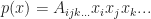
Which allows us to reinterpret p as a “r-multilinear function” on x. We say that a function $f(x_0, x_1, ..., x_{d-1} )$ is multilinear if for any of its arguments $x_i$ , it is a linear function, that is:

$f(x_0, x_1, ... a x_i + y, .... x_{d-1}) = af(x_0, x_1, ... x_i, .... x_{d-1}) + f(x_0, x_1, ... y, .... x_{d-1})$

While it may seem a bit restrictive to work in homogeneous polynomials only, in practice it doesn’t make much difference. Here is a simple trick that ought to be familiar to anyone in computer graphics who knows a bit about projective matrices. Let us consider the following 1D example (which trivially generalizes): given a polynomial in one variable,

$p(x) = a_0 + a_1 x + a_2 x^2$

Let us create a new variable $w$ , and construct the new polynomial:

$p'(x, w) = a_0 w^2 + a_1 xw + a_2 x^2 = w^2 p(\frac{x_0}{w})$

Now we observe that:

$p'(x,w)$ is a homogeneous polynomial of degree 2.
If we pick $w = 1$ , then $p'(x, 1) = p(x)$ .

And so we have faithfully converted our inhomogeneous degree 2 polynomial in one variable into a new homogeneous degree 2 polynomial in two variables!

In general, converting from an inhomogeneous polynomial to a homogeneous polynomial is a simple matter of adding an extra variable. The fully generalized version works like this: Suppose that we have a polynomial $p(x_0, x_1, ... x_{d-1})$ of degree r in d unknowns. Then we add a variable, w, and construct the new homogeneous degree r polynomial,

$p'(x_0, x_1, ... x_{d-1}, w) = w^r p( \frac{x_0}{w}, \frac{x_1}{w}, \frac{x_2}{w}, ...)$

And again, $p'(x_0, x_1, ... , 1) = p(x_0, x_1, ...)$ .

Indexing, iteration and combinatorics

So with that stuff above all out of the way, we shall now settle on an implementation: we’re going to use symmetric tensors to represent homogeneous polynomials. Let us start off by listing a few basic properties about symmetric tensors:

A tensor $A_{ijk...}$ is called symmetric if for all permutations of an index, $ijk..., jki...$ and so on, $A_{ijk...} = A_{jki...} = ...$ .
As a result, all vectors (aka a rank-1 tensors) are trivially symmetric.
Similarly, a matrix is symmetric if and only if $M_{ij} = M_{ji}$ .
A rank 3 tensor is symmetric if $M_{ijk} = M_{ikj} = M_{jik} = M_{jki} = M_{kij} = M_{kji}$ (and so on).
Consequently is the dimension of each of the indices in a symmetric tensor must be equal, and so we shall sometimes refer to this quantity as the “dimension of the tensor”, or when we need to be more specific we shall call it the index dimension.
The dimension of the space of all symmetric tensors with rank r and (index) dimension d is ${ r + d - 1 \choose d - 1 }$ .

And so the first problem that we must solve is to figure out how to pack the coordinates of a general rank r, dimension d symmetric tensor into an array of size ${ r + d - 1 \choose d - 1 }$ . Closely related to this issue is the problem of indexing, and we are going to need methods for both randomly accessing elements of the tensor and for performing sequential iteration over the unique entries. In fact, it is really this last issue which is the most essential, since if we can define an efficient method for enumerating the unique elements of the tensor, then we can simply use the order in which we enumerate the entries of the tensor as the indexes into a flat array.

By definition, the entries of a symmetric tensor are invariant under index permutation. This leads to two distinct ways to index into a symmetric rank r dimension d tensor:

Tensor style indexing – This is the ordinary way that we write the index for a generic tensor using subscripts. Entries of the tensor are parameterized by a length r vector of integers, $(i_0, i_1, ... i_{r-1})$ where $0 \leq i_k< d$ for all $0 \leq k < r$ .
Polynomial style (degree) indexing – This is the style of indexing is unique to symmetric tensors and comes from their close association with polynomials. Here, we take the index to be the degree of one of the monomial terms in the corresponding homogeneous polynomial These indices are enumerated by length d vectors of integers, $(a_0, a_1, ... a_{d-1})$ where $a_k \geq 0$ for all k, and $\sum \limits_{k=0}^{d-1} a_k = r$ .

We can convert between these two types of indexes up to a point. Converting from tensor indexing to degree indexing is straightforward, where we just pick

$a_k =$ the number of elements in $(i_0, ... i_{r-1})$ that are equal to k

Going the other way is a bit harder, since there are multiple tensor indices which map to the same degree index. To resolve the ambiguity, we can simply take the lexicographically first item. This same idea also turns out to be useful for enumerating the entries within our tensor. For example, suppose that we wanted to enumerate the components of a rank 3, degree 4 tensor. Then, we could use the following ordering,

Pos.   Tensor   Degree
-------------------------
0      (0,0,0)  (3,0,0,0)
1      (1,0,0)  (2,1,0,0)
2      (2,0,0)  (2,0,1,0)
3      (3,0,0)  (2,0,0,1)
4      (1,1,0)  (1,2,0,0)
5      (2,1,0)  (1,1,1,0)
6      (3,1,0)  (1,1,0,1)
7      (2,2,0)  (1,0,2,0)
8      (3,2,0)  (1,0,1,1)
9      (3,3,0)  (1,0,0,2)
10     (1,1,1)  (0,3,0,0)
11     (2,1,1)  (0,2,1,0)
12     (3,1,1)  (0,2,0,1)
13     (2,2,1)  (0,1,2,0)
14     (3,2,1)  (0,1,1,1)
15     (3,3,1)  (0,1,0,2)
16     (2,2,2)  (0,0,3,0)
17     (3,2,2)  (0,0,2,1)
18     (3,3,2)  (0,0,1,2)
19     (3,3,3)  (0,0,0,3)

Here, the left hand column represents the order in which the entries of the tensor were visited, while the middle column is the set of unique tensor indices listed lexicographically. The right hand side is the corresponding degree index, which is remarkably in colexicographic order! This suggests other interesting patterns as well, such as the following little theorem:

Proposition: Colexicographically sort all the degree indices in a rank r, d-dimensional symmetric tensor. Then the position of the degree index, $(a_0, a_1, ... a_{d-1})$ , is

$\sum \limits_{j=1}^n {{ j-1+\sum \limits_{k=n-j}^n a_k} \choose j}$

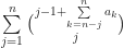
(That is supposed to be a binomial coefficient, but the parenthesis seem to be a bit messed up in wordpress.) I will leave this proof as an exercise to the reader, but offer the hint that it can be proven directly by induction. It is also interesting to note that the formula for the position does not depend on either the rank of the tensor or the first coefficient.

Putting it all together

Now let us try to work out a method for iterating the tensor index incrementally. A simple strategy is to use a greedy method: We just scan over the index until we find a component that can be incremented, then scan backwards and reset all the previous indices. In psuedo-C++, the code looks something like this:

bool next() {
  for(int i=0; i<rank; ++i) {
    if(tensor_index[i] < dimension - 1) {
      ++tensor_index[i];
      for(int j=i-1; j>=0; --j) {
          tensor_index[j] = tensor_index[i];
      }
      return true;
    }
  }
  return false;
}

The tensor_index array contains rank elements, and is initialized to all 0’s before this code is called. Each call to next() advances tensor_index one position.

Superficially, there are some similarities between this algorithm and the method for incrementing a binary counter. As a result, I propose the following conjecture (which I have not investigated carefully enough to say is true confidently):

Conjecture: Amortized over course of a full traversal, the cost of next is constant.

Using all this stuff, I’ve put together a little C++ class which iterates over the coordinates of a symmetric tensor. I’ve also uploaded it to github, where you can go download and play around with it (though it isn’t much). I hope to keep up this trend with future updates. For those who are curious, here is the URL:

https://github.com/mikolalysenko/0fpsBlog

Next time

In the next episode, I am going to continue on this journey and build an actual symmetric tensor class with a few useful operations in it. More speculatively, we shall then move on to rational mappings, algebraic surfaces, transfinite interpolation and deformable objects!

How to deal with polynomials?

Quick Review

Indexing, iteration and combinatorics

Putting it all together

Next time

Share this:

Like this:

Related

Leave a Reply Cancel reply