Smooth Voxel Terrain (Part 1)

My god… I’ve now written three blog posts about Minecraft. If you are at all like me, you may be getting just a bit tired of all those cubes. To avoid fatigue, I think now is a good time to change things up. So today let’s talk about something cool and different — like how to deal with smooth blobby shapes:

: A rendering of Goursat’s surface.

Blobby Objects

But before we get too far ahead of ourselves, we need to say what exactly a blobby object is. The term `blobby object’ is one of Jim Blinn’s many contributions to computer graphics, though some of the basic ideas go back much further. In fact mathematicians have known about blobs for centuries (before they even had calculus!) Conceptually, the basic idea of a blobby object is quite simple, though it can be a bit tricky to formalize it properly.

The theoretical basis for blobby object modeling is the concept of an implicit solid. The idea is that we can represent a solid object by a contour of a smooth function. I found the following beautiful picture from wikipedia that illustrates the concept:

: Public domain illustration of a 2D implicit set. (c) Wikimedia, created by Oleg Alexandrov.

Now we want to get a solid (that is a closed regular set) — not just any old sublevel set. Fortunately, the definition is pretty simple once you’ve seen it and get used to it. Given any continuous function, $f(x,y,z)$ , it determines a set which we call the regularized 0-sublevel,

$V_0(f) \stackrel{def}{=} \kappa f^{-1}([-\infty, 0)) = \kappa \{ (x,y,z) \in \mathbb{R}^3: f(x,y,z) < 0 \}$

(Here I’m using the symbol $\kappa$ to denote the closure operator.) Unpacked, this means that $V_0(f)$ is the closure (of the preimage of (the open interval $[-\infty, 0)$ ) ). Our definition of $V_0$ is a little bit different than the standard (but unfortunately slightly broken) definition which you see quite frequently:

$Z_0(f) \stackrel{def}{=} f^{-1}( [-\infty, 0] ) = \{ (x,y,z) \in \mathbb{R}^3 : f(x,y,z) \leq 0 \}$

Spiritually, this is the right idea but technically it doesn’t quite work. It is true that in many situations, these two definitions give similar results. For example, let’s consider the 1D function $f(x) = x^2 - 1$ . This has a pair of roots at $\pm 1$ , and looks like this:

In this case, both $Z_0(f)$ and $V_0(f)$ will give us the same result, that is the interval $[-1, 1]$ . Where things break down however is near the edge cases. If for example we took the function $f(x) = x^2$ :

Then $Z_0(f)$ would give us a point while $V_0(f)$ is empty! Now you might ask, why should we prefer one definition over the other. There are at least a couple good reasons:

First, $Z_0$ is not necessarily a solid. This means that it is not always uniquely determined by its boundary, and that certain mass properties (like volume, inertia, momentum, etc.) may fail to be well defined. On the other hand, $V_0$ is always a nice solid object, and so we don’t ever have to worry about such pathologies.
Closely related to the first point, it is very difficult to define regularized Boolean operation on the latter representation, while it is possible to perform CSG operations regularized sublevels using Rvachev functions. (Maybe I will say more about this at some point in the future.)
Finally, it is not even practically possible to numerically compute $Z_0$ anyway! The reason for this is that most general purpose methods for finding 0-sets use sampling to check for places where f crosses the 0-axis (this is an application of the intermediate value theorem from calculus). If we include these isolated 0 points in our definition, then we are in the hopeless situation where we must be infinitely lucky to get one of our sample points to even detect them! (And if you get really unlucky and one of them actually does show up, then there is a good chance your code might even break if you are using the $Z_0$ definition!)

To boil all this down to a pithy remark:

The reason we prefer $V_0$ over $Z_0$ is that it detects 0-crossings — not 0-values!

My personal reason for preferring $V_0$ over $Z_0$ is that it is what is actually used in practice anyway. In fact, even when most people say they are using $Z_0$ , what they end up actually computing is $V_0$ , because the only thing they can actually compute are the crossings!

Isosurface Extraction

Now that we’ve hopefully got a decent mental picture of what we want to find, let’s try to figure out how to compute something with it. In particular, we are most interested in finding the boundary of the implicit set. An obvious application would be to draw it, but knowing the boundary can be equally useful for other tasks as well; like computing mass properties for example.

In light of our previous definition, the boundary of our implicit solid is going to be the set of all 0-crossings of f. One perspective is that computing the boundary is like a higher dimensional generalization of root finding. Thinking metaphorically for a moment and confusing 0-values with 0-crossing, it is like saying that instead of trying to find solutions for:

$f(x) = 0$

We are now looking for all solutions to the more general problem:

$f(x,y,z) = 0$

In the first case, we get some points as an output, while in the second case the solution set will look like some surface.

Implicit Function Theorem

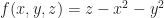
It turns out that at least when f is smooth, we can convert implicit sets locally into parametric surfaces. This is the content of the implicit function theorem. Finding such a parametric surface is as good as solving the equation. For example, say we had a paraboloid given by:

$f(x,y,z) = z - x^2 - y^2$

Then we could parameterize the 0-set by the surface:

$x(u,v) = u$

$y(u,v) = v$

$z(u,v) = u^2 + v^2$

When you have a parametric solution, life is good. Unfortunately, for more complicated equations (like Perlin noise for example), finding a parametric solution is generally intractable. It also doesn’t work so well if your implicit function happens to come from some type of sampled geometry, such as a distance field or a point cloud. As a result, exact parametric solutions are generally too much to hope for.

Ray Tracing

A more general solution to the problem of isosurface extraction is ray tracing, which is basically a form of dimensionality reduction. The idea is that instead of trying to find the whole isosurface, we instead just look to query it locally. What we do is define some ray (or more generally any curve) $\varphi : [0,1] \to \mathbb{R}^3$ , and then try to solve for the place where f composed with $\varphi$ crosses 0:

$f( \varphi(t) ) = 0$

This is now a standard 1D root-finding problem, and we could solve it using either symbolically or using techniques from calculus, like bisection or Newton’s method. For example, in path tracing, one usually picks a collection of rays corresponding to the path light would take bouncing through the scene. Then all we need to do is check where these individual rays meet the surface, rather than compute the entire thing all at once (though it can still become very expensive).

Meshing

For most interesting functions, it is neither possible to find a parametric description, nor is ray tracing really fast enough. Instead, it is often more practical to look at finding some polygonal approximation of the implicit surface instead. Broadly speaking, this process has two parts:

First, we approximate $f$ by sampling
Then, from this sampled version of $f$ , we try to find some mesh which approximates $f = 0$ .

Of course there are many details hidden within this highly abstract description. I wrote up a fairly lengthy exposition, but ended up more than tripling the length of this post! So, I think now is a good time to take a break.

Next Time

Next time we’ll talk about how to put all this stuff into practice. The focus is going to be on meshing, since this is probably the most important thing to deal with in practice. As a sneak preview of things to come, here is a demo that I put together. I promise all (well ok at least something) will be explained in the coming post!

Smooth Voxel Terrain (Part 1)

Blobby Objects