Conway’s Game of Life is one of the most popular and iconic cellular automata. It is so famous that googling it loads up a working simulation right in your browser! The rules for the Game of Life (GoL) can be stated in a few lines:
- The world is an infinite rectangular array of cells, each of which can be in one of two states: alive or dead; and the neighborhood of each cell is a 3×3 grid centered on the cell.
- The state of the world advances in discrete synchronous time steps according to the following two rules:
- Cells which are alive remain alive if and only if they have between 2 and 3 neighbors; otherwise they die.
- Cells which are dead become alive if they have exactly 3 neighbors; or else they stay dead.
Despite the superficial simplicity of these rules, the Game of Life can produce many unexpected and fascinating recurring patterns; like the glider soliton:

The fact that the rules for the Game of Life are so short and clear makes it a great project for initiating novice programmers. Since Life was invented by John Conway in 1970, it has distracted many amateur and recreational mathematicians, leading to the discovery of many interesting patterns. For example, Paul Chapman showed that Life is Turing complete, and so it is in principle possible to translate any computer into a set of initial conditions. As an amusing example of this concept, here is an implementation of Conway’s Game of Life in the Game of Life created by Brice Due. Another cool pattern is the famous Gemini spaceship which is a complex self replicating system, and is perhaps the first true `organism’ to be discovered in life! If any of this sounds interesting to you, you can play around with the Game of Life (and some other cellular automata) and look at a large and interesting library of patterns collected in the community developed Golly software package.
SmoothLife
Now, if you’ve been programming for any reasonable length of time you’ve probably come across the Game of Life at least a couple of times before and so all the stuff above is nothing new. However, a few weeks ago I saw an incredibly awesome video on reddit which inspired me to write this post:
This video is of a certain generalization of Conway’s Game of Life to smooth spaces proposed by Stephan Rafler:
S. Rafler, “Generalization of Conway’s “Game of Life” to a continuous domain – SmoothLife” (2011) Arxiv: 1111.1567
You can read this paper for yourself, but I’ll also summarize the key concepts here. Basically, there are two main ideas in Rafler’s generalization: First, the infinite grid of cells is replaced with an `effective grid’ that is obtained by averaging over a disk. Second, the transition functions are replaced by a series of differential equations derived from a smooth interpolation of the rules for the discrete Game of Life.
Effective Grids
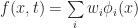
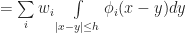
To explain how an `effective grid’ works, first consider what would happen if we replaced the infinite discrete grid in the game of life with a time-dependent continuous real scalar field, 
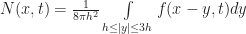
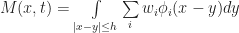
Now for each cell, we also want to compute the effective “number of cells” in its neighborhood. To do this, we use the same averaging process, only over a larger annulus centered at x. By analogy to the rules in the original GoL, a reasonable value for the outer radius is about 3h. Again, following Rafler’s conventions we call this quantity N(x,t):
To illustrate how these neighborhoods fit together, I made a small figure:

Now there are two things to notice about M and N:
- They are invariant under continuous shifts.
- They are invariant under rotations.
This means that if we define the state of our system in terms of these quantities, the resulting dynamics should also be invariant under rotations and shifts! (Note: These quantities are NOT invariant under scaling, since they are dependent on the choice of h.)
Smooth Transition Functions
Of course getting rid of the grid is only the first step towards a smooth version of Life. The second (and more difficult) part is that we also need to come up with a generalization of the rules for the game of life that works for continuous values. There are of course many ways to do this, and if you’ve taken a course on real analysis you may already have some idea on how to do this. However, for the sake of exposition, let’s try to follow along Rafler’s original derivation.
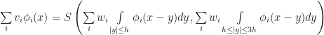
As a starting point, let’s first write the rules for the regular discrete Game of Life in a different way. By some abuse of notation, suppose that our field f was a discrete grid (ie 

Where S represents the transition function of the Game of Life, and is defined to be:
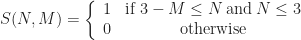
Since S is a function of two variables, we can graph it by letting the x-axis be the number cells in the neighborhood and the y-axis be the state of the cell:
Now given such a representation, our task is to `smooth out’ S somehow. Again to make things consistent with Rafler, we first linearly rescale N, M so that they are in the range [0,1] (instead of from [0,9), [0,2) respectively). Our goal is to build up a smooth approximation to S using sigmoid functions to represent state transitions and thresholding (this is kind of like how artificial neural networks approximate discrete logical functions). Of course the term `sigmoid’ is not very precise since a sigmoid can be any function which is the integral of a bump. Therefore, to make things concrete (and again stay consistent with Rafler’s paper) we will use the logistic sigmoid:
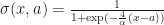
It is a bit easier to understand what 


 from x = -6 to 6. Image (c) Wikipedia 2008. Author Geoff Richards.
Intuitively, 

The idea is that we think of effective field values greater than 0.5 as a live, and those less than 0.5 as dead. We can also adapt this idea to smoothly switch between any two different values depending on whether a cell is alive or dead:

The idea is that 


 for n=0 to 1
Putting it all together, let’s now make a state transition function which selects the corresponding interval based on whether the state of the cell is currently alive or dead:

Where ![[b_1, d_1], [b_2, d_2]](https://s0.wp.com/latex.php?latex=%5Bb_1%2C+d_1%5D%2C+%5Bb_2%2C+d_2%5D&bg=ffffff&fg=1a1a1a&s=0&c=20201002)
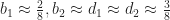

This is the transition function for SmoothLife as defined by Rafler. The squishing of this plot relative to the original plot is just a side effect of rescaling the axes to the unit interval, but even so the similarity is unmistakable. The only thing left is to pick the value of 


Timestepping
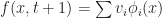
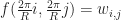
Now, there is still one nagging detail. I have not yet told you how the time works in this new version of life. In Rafler’s paper he gives a couple of possibilities. One simple option is to just do discrete time stepping, for example:

However, this has the disadvantage that the time stepping is now discretized, and so it violates the spirit of SmoothLife somewhat. Another possibility (advocated in Rafler’s paper) is to rewrite this as a differential equation, giving the following smooth update rule:
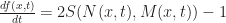
I found this scheme to give poor results since it tends to diverge whenever the state of a cell is relatively stable (leading to field values outside the range [0,1]). (UPDATE: I just got an email from Stephan Rafler, apparently the equation I wrote earlier was wrong. Also, he recommends that the field values be clamped to [0,1] to keep them from going out of bounds.) A slightly better method which I extracted from the source code of SmoothLife is the following technique that pushes the state of the effective field towards S exponentially:

It is also possible to replace f(x,t) with M(x,t) on the right hand side of the above equations and get similar results. It is claimed that each of these rules can produce interesting patterns, though personally I’ve only observed the first and last choices actually working…
Discretizing SmoothLife
Now that we have the rules for SmoothLife, we need to figure out how to actually implement it, and to do this we need to discretize the field f somehow. One common way to do this is to apply the Galerkin method. The general idea is that for a fixed t, we write f as a weighted sum of simpler basis functions 
The undetermined weights 


Well given that 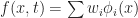

To compute M we just plug in f(x,t):
And a similar formula holds for N as well. Therefore, we have the equation:
Unfortunately, it is usually not the case that there is an exact solution to this equation. The underlying reason the above idea may fail is that it might not be possible to represent our solution in the basis functions 
Minimize

This type of system is sometimes called the weak formulation of the boundary value problem, and by standard linear algebra arguments finding the solution amounts to doing a subspace projection. In general this could be pretty annoying, but if we suppose that each of our
Then we know that,

and so all we have to do to compute the next state is integrate S(N,M) against each
Boundary Conditions
Ok, so we know (at least theoretically) what must be done to discretize the system. But how can we possibly hope to represent an infinite space using a finite number of basis functions? One simple solution is that we can make the space finite again by adding a periodicity condition. That is, let us require that for all x,y:

This means that we can parameterize the state of the infinite grid by just describing what happens within the region 
Sinc Interpolation
Finally, we come to the point where we must pick a basis in order to go any further. There is some level at which the particular choice of representative functions
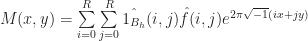
However, because our system is periodic and translationally invariant (although not linear) there is one basis which has at least a somewhat more special status, and that is the Dirichlet or aliased sinc basis. Let R be the resolution of a uniform grid, and define:
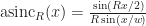
Then we index our basis functions by a pair of indices 

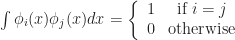
It may seem surprising at first, but these basis functions are actually orthogonal. If you’ve never seen something like this before, please don’t be alarmed! That definition (which seemed to come out of left field) is really a manifestation of the famous (and often misunderstood) Nyquist sampling theorem. It basically says that if we write any periodic, band limited function as a sum of sincs:

Then the weights 
This means that for any suitably smooth f, we can project it to our basis by just sampling it:

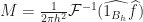
This makes our code way simpler, since we can avoid doing some messy numerical integration to get the weights. Assuming that S(N,M) is smooth enough (which in practice it is), then all we have to do to perform a discrete update is figure out how to compute M(x,y), N(x,y) for any given sinc expansion of f. In other words, we want to compute:

But this is just a convolution convolution with the indicator function of the unit disk:

If you know a bit of Fourier analysis, you should know what comes next. Just take a Fourier transform and apply the convolution theorem to both sides, giving:

Which we can actually solve exactly, since the Nyquist theorem implies that 
And by a bit of calculus, the Fourier transform of 
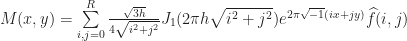
A similar formula for N(x,y,t) can be obtained by writing:

Putting it all together, let 

I’ll leave it as an exercise to work out the update rules for the continuous time steps.
Implementation Details
Great, so we have some formulas for computing the next time step, but if we do it in a dumb way it is going to be pretty slow. The reason is that each of the above steps requires summing up all the coefficients of f to calculate M and N at each point, which is going to take linear work with respect to the number of terms in our summation. Spread out over all the points in the grid, this makes the total update 
- Initialize f
- Precalculate
- For t=1 to n
- Use FFT to compute
- Set
- Set
- Set
- Use FFT to compute


And that’s it!
Demo
If you want to try out SmoothLife yourself in your browser, I made a few jsFiddles which illustrate the basic principle. Here is a Fourier based implementation that follows the discussion in this article pretty closely:
http://jsfiddle.net/mikola/aj2vq/
I also made a second WebGL/GPU based implementation that uses a discretization similar to that proposed in Rafler’s original paper:
http://jsfiddle.net/mikola/2jenR/
You can run either of them in your browser and try changing the parameters.
Next Time…
The stuff in this article is basically background material, and most of it can be found in Rafler’s paper or is already more-or-less documented in the source code for the SmoothLife project on SourceForge. However, in the sequel I plan to go a bit farther than the basic rules for SmoothLife and tell you how to make a version of SmoothLife for curved surfaces!

Fantastic explanation. Can’t wait to see the description for curved surfaces. Will you work on a coordinate-free representation of a mesh, or on an explicit embedding?
Coordinate free. Technically the only thing we need is a Riemannian metric to compute the effective fields M and N. The basic generalization is actually quite simple (if you know a bit of geometry anyway), but the difficult part is actually discretizing and implementing it correctly. I was originally planning on covering the whole thing in one post, but it got a bit long and I decided to break it into two parts.
The glider for the smooth system is pretty cool 🙂
For a while I have thought of using it as a replacement for the conventional Life glider as a symbol for hackerdom (as popularized by ESR) for those who would rather not link to ESR’s page on the symbol.
Great work! I especially liked your detailed explanation of the discretization process. One question though: do you know why your version doesn’t seem to exhibit the “connecting rods” that go between the blobs that are the glider equivalents?
The reason it does not is that the connecting rod version uses a different time stepping scheme and parameters. The parameters I linked to are the same as those described in Rafler’s original paper, and are known to produce gliders/solitons.
I like some of these slow-moving ones: http://jsfiddle.net/XgusZ/
I love these patterns: http://jsfiddle.net/Dn3xL/
I could play with this for hours… http://jsfiddle.net/6DkJJ/
I’m glad you like it!
Now can someone build a turing machine in it? 😉
this is WEIRD! : it uses Conway GOL for tiling http://www.logarithmic.net/ghost.xhtml
Thhanks great blog
Your code does not match the article at all. I want to understand every step of the implementation process, and your code is impossible to navigate. Like, why is your BesselJ() method set up the way it is? The article does not explain this well.
I haven’t touched this in years, and it also looks like JSFiddle no longer correctly renders those examples. Reading the code it looks like the BesselJS function is precomputing the Fourier multiplier numerically. I think the reason I did it that way was that it was simpler than trying to compute the exact normalization coefficients for the DFT since this is all handled implicitly by the FFT/inverse FFT itself. Once you have the multiplier, getting those neighborhood counts is a just an application of the convolution theorem.
I’m just trying to relate your code to the article. So is the multiplier in BesselJ() that you referred to the Fourier transform of the indicator function?