Collision detection (part 2): Box intersection

Last time, we discussed collision detection in general and surveyed some techniques for narrow phase collision detection.  In this article we will go into more detail on broad phase collision detection for closed axis-aligned boxes.  This was a big problem in the 1970’s and early 1980’s in VLSI design, which resulted in many efficient algorithms and data structures being developed around that period.  Here we survey some approaches to this problem and review a few theoretical results.

Boxes

A box is a cartesian product of intervals, so if we want to represent a d-dimensional box, it is enough to represent a tuple of d 1-dimensional intervals.  There are at least two ways to do this:

• As a point with a length
• As a pair of upper and lower bounds

For example, in 2D the first form is equivalent to representing a box as a corner point together with its width and height (e.g. left, top, width, height), while the second is equivalent to storing a pair of bounds (e.g. ).

To test if a pair of boxes intersect, it is enough to check that their projections onto each coordinate axes intersects. This reduces the d-dimensional problem of box intersection testing to the 1D problem of detecting interval overlap.  Again, there are multiple ways to do this depending on how the intervals are represented:

• Given two intervals represented by their center point and radius, ,

• Given two intervals represented by upper and lower bounds, ,

In the first predicate, we require two addition operations, one absolute value and one comparison, while the second form just uses two comparisons.  Which version you prefer depends on your application:

1. In my experiments, I found that the first test was about 30-40% faster in Chrome 39 on my MacBook, (though this is probably compiler and architecture dependent so take it with a grain of salt).
2. The second test is more robust as it does not require any arithmetic operations.  This means that it cannot fail due to overflow or rounding errors, making it more suitable for floating point inputs or applications where exact results are necessary.  It also works with unbounded (infinite) intervals, which is useful in many problems.

For applications like games where speed is of the utmost importance, one could make a case for using the first form.  However, in applications where it is more important to get correct results (and not crash!) robustness is a higher priority.  As a result, we will generally prefer to use the second form.

1D interval intersection

Before dealing with the general case of box intersections in d-dimensions, it is instructive to look at what happens in 1D.  In the 1D case, there is an efficient sweep line algorithm to report all intersections.  The general idea is to process the end points of each interval in order, keeping track of all the intervals which are currently active.  When we reach the start of a new interval, we report intersections with all currently active intervals and it to the active set, and when we reach the end of an interval we delete the interval from the active set:

In JavaScript, it looks something like this:

function sweepIntervals(intervals) {
  var events = [], result = [], active = []
  intervals.forEach(function(interval, id) {
    events.push(
      { t: interval[0], id: id, create: 1 },
      { t: interval[1], id: id, create: 0 })
  })
  events.sort(function(a, b) {
    return a.t - b.t || b.create - a.create
  })
  events.forEach(function(ev) {
    if(ev.create) {
      active.forEach(function(id) {
        result.push([ev.id, id])
      })
      active.push(ev.id)
    } else
      active.splice(active.indexOf(ev.id), 1)
  })
  return result
}

If the number of intervals is , then there are events total, and so sorting them all takes time.  Processing event requires a scan through the active set, however for each iteration one intersecting pair is reported.  If the total number of collisions is , then the amortized cost of looping over the events is .  Therefore, the total running time of this algorithm is in .

Sweep and prune

Sweeping is probably the best solution for finding interval overlaps in 1D.  The challenge is to generalize this to higher dimensions somehow.  One approach is to just run the 1D interval sweep to filter out collisions along some axis, and then use a brute force test to filter these pairs down to an exact set,

In JavaScript, here is an illustration of how it could be implemented in terms of the previous 1D sweep algorithm:

//Assume each box is represented by a list of d intervals
//Each interval is of the form [lo,hi]
function sweepAndPrune(boxes) {
  return sweepIntervals(boxes.map(function(box) {
    return box[0]
  }).filter(function(pair) {
    var A = boxes[pair[0]], B = boxes[pair[1]]
    for(var i=1; i<A.length; ++i) {
      if(B[i][1] < A[i][1] || A[i][1] < B[i][0])
        return false
    }
    return true
  })
}

The germ of this idea is contained in Shamos and Hoey’s famous paper on geometric intersection problems,

M. Shamos, D. Hoey (1976) “Geometric intersection problems” FoCS

In the case of rectangles in the plane, one can store the active set in an interval tree (more on this later), giving an optimal algorithm for planar intersection of rectangles.  If we just store the active set as an array, then this technique is known as sweep-and-prune collision detection, which is widely used in packages like I-COLLIDE,

J. Cohen, M. Lin, D. Manocha, M. Ponamgi. (1995) “I-COLLIDE: An interactive and exact collision detection system for large-scale environments” Symposium on Interactive 3D Graphics

For objects which are well separated along some axis, the simple sweep-and-prune technique is very effective at speeding up collision detection.  However, if the objects are grouped together, then sweep-and-prune is less effective, realizing a complexity no better than brute force .

Uniform grids

After brute force, grids are one of the simplest techniques for box intersection detection.  While grids have been rediscovered many times, it seems that Franklin was one of the first to write extensively about their use in collision detection,

W. Franklin (1989) “Uniform grids: A technique for intersection detection on serial and parallel machines” Proceedings of Auto-Carto

Today, grids are used for many different problems, from small video games all the way up to enormous physical simulations with millions of bodies.  The grid algorithm for collision detection proceeds in two phases; first we subdivide space into uniformly sized cubes of side length , then insert each of the boxes into the cells they overlap.  Boxes which share a common grid cell are tested for overlaps:

Implementing a grid for collision detection is only just more complicated than sweep and prune:

//Same convention as above, boxes are list of d intervals
// H is the side length for the grid
function gridIntersect2D(boxes, H) {
  var grid = {}, result = [], x = [0,0]
  boxes.forEach(function(b, id) {
    for(x[0]=Math.floor(b[0][0]/H); x[0]<=Math.ceil(b[0][1]/H); ++x[0])
    for(x[1]=Math.floor(b[1][0]/H); x[1]<=Math.ceil(b[1][1]/H); ++x[1]) {
      var list = grid[x]
      if(list) {
        list.forEach(function(otherId) {
          var a = boxes[otherId]
          for(var i=0; i<2; ++i) {
            var s = Math.max(a[i][0], b[i][0]),
                t = Math.min(a[i][1], b[i][1])
            if(t < s || Math.floor(s/H) !== x[i])
              return
          }
          result.push([id, otherId])
        })
        list.push(id)
      } else grid[x] = [id]
    }
  })
  return result
}

Note here how duplicate pairs are handled:  Because in a grid it is possible that we may end up testing the same pair of boxes against each other many times, we need to be careful that we don’t accidentally report multiple pairs of collisions.  One way to prevent this is to check if the current grid cell is the lexicographically smallest cell in their intersection.  If it isn’t, then we skip reporting the pair.

While the basic idea of a grid is quite simple, the details of building efficient implementations are an ongoing topic of research.  Most implementations of grids differ primarily in how they manage the storage of the grid itself.  There are 3 basic approaches:

• Dense array:  Here the grid is encoded as a flat array of memory.  While this can be expensive, for systems with a bounded domain and a dense distribution of objects, the fast access times may make it preferable for small systems or parallel (GPU) simulations.
• Hash table:  For small systems which are more sparse, or which have unbounded domains, a hash table is generally preferred.  Accessing the hash table is still , however because it requires more indirection iterating over the cells covering a box may be slower due to degraded data locality.
• Sorted list: Finally, it is possible to skip storing a grid as such and instead store the grid implicitly.  Here, each box generates a cover of cells which are then appended to a list which is then sorted.  Collisions correspond to duplicate cells which can be detected with a linear scan over the sorted list. This approach is easy to parallelize and has excellent data locality, making it efficient for systems which do not fit in main memory or need to run in parallel.  However, sorting is asymptotically slower than hashing, requiring an extra overhead, which may make it less suitable for problems small enough to fit in RAM.

Analyzing the performance of a grid is somewhat tricky.  Ultimately, the grid algorithm’s complexity depends on the distribution of boxes.  At a high level, there are 3 basic behaviors for grids:

• Too coarse: If the grid size is too large, then it won’t be effective at pruning out non-intersecting boxes.  As a result, the algorithm will effectively degenerate to brute force, running in .
• Too fine: An even worse situation is if we pick a grid size that is too small.  In the limit where the grid is arbitrarily fine, a box can overlap an infinite number of cells, giving the unbounded worst case performance of !!!
• Just right:  The best case scenario for the grid is that the objects are uniformly distributed in both space and size.  Ideally, we want each box to intersect at most cells and that each cell contains at most objects. In this case, the performance of a grid becomes  (using a grid or hash table), or for sorted lists, which for small is effectively an optimal complexity.

Note that these cases are not mutually exclusive, it is possible for a grid to be both too sparse and too fine at the same time. As a result, there are inputs where grids will always fail, no matter what size you pick.  These difficulties can arise in two situations:

• Size variation:  If the side lengths of the boxes have enormous variability, then we can’t pick just one grid size.  Hierarchical grids or quad trees are a possible solution here, though it remains difficult to tune parameters like the number of levels.
• High aspect ratio: If the ratio of the largest to smallest side of the boxes in the grid is too extreme, then grids will always fail catastrophically.  There is no easy fix or known strategy to avoid this failure mode other than to not use a grid.

While this might sound pessimistic, it is important to remember that when grids work they are effectively optimal.  The trouble is that when they fail, it is catastrophic.  The bottom line is that you should use them only if you know the distribution of objects will be close to uniform in advance.

Partition based data structures

After grids, the second most widely recommended approach to collision detection are partition based tree data structures.  Sometimes called “bounding volume hierarchies,” partition based data structures recursively split space into smaller regions using trees. Objects are iteratively tested against these trees, and then inserted into the resulting data structure.

In psuedo-JavaScript, here is how this algorithm works:

function bvhIntersect(boxes) {
  var tree = createEmptyTree(), result = []
  boxes.forEach(function(box, id) {
    bvhQuery(tree, box).forEach(function(otherBox) {
      result.push([box, otherBox])
    })
    bvhInsert(tree, box)
  })
  return result
}

While the insertion procedure is different for each tree-like data structure, in bounding volume hierarchies querying always follows the same general pattern: starting from the root of the tree, recursively test if any children intersect the object.  If so, then visit those children, continuing until the leaves of the tree are reached.  Again, in psuedo-JavaScript:

function bvhQuery(node, box) {
  if(!node.bounds.intersects(box))
    return []
  if(isLeaf(node))
    return [ node.item ]
  return node.children.reduce(function(child, result) {
    return result.concat(bvhQuery(child, box))
  }, [])
}

The precise complexity of this meta-algorithm depends on the structure of the tree, the distribution of the boxes and how insertion is implemented.  In the literature, there are many different types of bounding volume hierarchies, which are conventionally classified based on the shape of the partitions they use.  Some common examples include:

• kd-trees:  Axis aligned hyperplane
• R-trees (aka AABB trees, box-trees): Axis aligned boxes
• OBB trees: Oriented boxes/slabs
• Sphere trees: Balls
• BSP trees: Hyperplanes

Within each of these general types of trees, further classification is possible based on the partition selection strategy and insertion algorithm.  One of the most comprehensive resources on such data structures is Samet’s book,

H. Samet. (2006) “Foundations of multidimensional and metric data structures“

Lower bounds

It would seem like the above description is too vague to extract any meaningful sort of analysis.  However, it turns out that using only a few modest assumptions we can prove a reasonable lower bound on the worst case complexity of bvhIntersect.  Specifically, we will require that:

1. The size of a tree with items is at most bits.
2. Each node of the tree is of bounded size and implemented using pointers/references.  (As would be common in Java for example).
3. Querying the tree take time, where is the number of items in the tree.

In the case of all the aforementioned trees these conditions hold.  Furthermore, let us assume that insertion into the tree is “cheap”, that is at most polylogarithmic time; then the total complexity of bvhIntersect is in the worst case,

.

Now here is the trick:  using the fact that the trees are all made out of a linear number of constant sized objects, we can bound the complexity of querying by a famous result due to Chazelle,

B. Chazelle. (1990) “Lower bounds for orthogonal range search I: The reporting case” Journal of the ACM

More specifically, he proved the following theorem:

Theorem: If a data structure answers box intersection queries in time, then it uses at least bits.

As a corollary of this result, any (reasonable) bounding volume hierarchy takes at least time per query.  Therefore, the worst case time complexity of bvhIntersect is slower than,

.

Now this bound does come with a few caveats.  Specifically, we assumed that the query overhead was linear in the number of reported results and neglected interactions with insertion.  If is practically , then it is at least theoretically possible to do better.  Again, we cite a result due to Chazelle, which shows that it is possible to report rectangle intersection queries in time using space,

B. Chazelle, (1988) “A functional approach to data structures and its use in multidimensional searching” SIAM Journal of Computing

R-trees

Finally, let us look at one particular type of bounding volume hierarchy in detail; specifically the R-tree.  Originally invented by Guttmann, R-trees have become widely used in GIS databases due to their low storage overhead and ease of implementation,

A. Guttmann, (1984) “R-Trees: A dynamic index structure for spatial searching” SIGMOD

The high level idea behind an R-tree is to group objects together into bounding rectangles of increasing size.  In the original paper, Guttmann gave several heuristics for construction and experimentally validated them.  Agarwal et al. showed that the worst case query time for an R-tree is and gave a construction which effectively matches this bound,

P.K. Agarwal, M de Berg, J. Gudmundsson, M. Hammar, H.J. Haverkort. (2002) “Box-trees and R-trees with near optimal query time” Discrete & Computational Geometry

Disappointingly, this means that in the worst case using R-trees as a bounding volume hierarchy gives an overall time complexity that is only slightly better than quadratic. For example in 2D, we get , and for 3D .

Still, R-trees are quite successful in practice.  This is because for cases with smaller query rectangles the overhead of searching in an R-tree approaches .  Situations where the complexity degenerates to tend to be rare, and in practice applications can be designed to avoid them.  Moreover, because R-trees have small space overhead and support fast updates, they are relatively cheap to maintain as an index. This has lead to them being used in many GIS applications, where the problem sizes make conserving memory the highest priority.

Range tree based algorithms

So far none of the approaches we’ve seen have managed to break the barrier in the worst case (with the exception of 1D interval sweeping and a brief digression into Shamos & Hoey’s algorithm).  To the best of my knowledge, all efficient approaches to this problem make some essential use of range trees.  Range trees were invented by Bentley in 1979, and they solve the orthogonal range query problem for points in time using space  (these results can be improved somewhat using fractional cascading and other more sophisticated techniques).  The first application of range tree like ideas to rectangle intersections was done by Bentley and Wood,

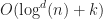
J. Bentley, D. Wood. (1980) “An optimal worst case algorithm for reporting intersections of rectangles” IEEE Transactions on Computers

In this paper they, introduced the concept of a segment tree, which solves the problem of interval stabbing queries.  One can improve the space complexity of their result in 2D using an interval tree instead, giving a algorithm for detecting rectangle intersections.  These results were generalized to higher dimensions and improved by Edelsbrunner in a series of papers,

H. Edelsbrunner. (1983) “A new approach to rectangle intersections I” International Journal of Computer Math

H. Edelsbrunner. (1983) “A new approach to rectangle intersections II”  International Journal of Computer Math

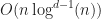
Amongst the ideas in those papers is the reduction of the intersection test to range searching on end points.  Specifically, it is true that if two 1D intervals intersect, then at least one of them contains the end points of the other box.  The recursive application of this idea allows one to use a range tree to resolve box intersection queries in 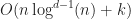dimensions using space and time.

Streaming algorithms

The main limitation of range tree based algorithms is that they consume too much space. One way to solve this problem is to use streaming.  In a streaming algorithm, the tree is built lazily as needed instead of being constructed in one huge batch.  If this is done carefully, then the box intersections can be computed using only extra memory (or even if we allow in place mutation) instead of .  This approach is described in the following paper by Zomorodian and Edelsbrunner,

A. Zomorodian, H. Edelsbrunner (2000) “A fast software for box intersections” SoCG

In this paper, the authors build a segment tree using the streaming technique, and apply it to resolve bipartite box interactions.  The overall time complexity of the method is 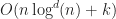, which matches the results for segment trees.

Next time

In the next part of this series we will look at some actual performance data from real benchmarks for each of these approaches.  Stay tuned!